

public and internal comparisons
across 12 ranked comparisons
Overview
Engineering work spans material and process data, design parameters, simulation meshes, particle states and physical tests. A useful engineering AI system must work across these representations and connect prediction with the decisions that follow: understanding influential inputs, comparing designs and choosing the next simulation or experiment.
Physics AI is increasingly demonstrating the value of learned models for accelerating individual simulation tasks. This report examines a broader question: can one probabilistic model family perform competitively across fundamentally different engineering and physical systems while remaining practical on workstation hardware? We test that proposition across fourteen benchmark tasks and studies in tabular learning, fluid dynamics, structural mechanics and optimization.
What makes DIM-GP different
DIM-GP is the model family within STOCHOS. Across this report, it operates on tables, unstructured meshes and particle states, including steady and transient physical systems. Its predictions are probabilistic and include uncertainty estimates; the same modeling framework connects prediction with sensitivity analysis and Bayesian optimization.
STOCHOS can incorporate inexpensive physical priors, multi-fidelity data and automatically calculated geometric features. STOCHOS Flow connects these capabilities to simulation tools and Python through visual workflows, supports foundation models and agentic AI workflows, and turns trained models into prediction applications for engineering teams.
The reported DIM-GP models were trained in less than one day, with less than 8 GB of GPU memory and at most one consumer GPU per run. Together, these capabilities form a general probabilistic modeling foundation for understanding, predicting and optimizing engineering systems.
Evidence across different problem representations
- Unstructured meshes and industrial physics — six PLAID boards. Top three on all six boards examined, including three first places.
- Particle states and transient dynamics — LagrangeBench. Lower error than the best of three published baselines in 19 of 21 dataset–metric comparisons.
- Large 3D surface meshes — AhmedML and DrivAerML. Lowest reported error across all seven evaluated channels in the ten-method comparisons.
- Tabular engineering data — TabArena-51 and TALENT-300. Third among 80 model entries on TabArena; lowest average rank in each task type when added to TALENT’s published comparison.
- Decisions under uncertainty — Bayesian optimization. 149 successful formulations in 150 runs in the virtual concrete study.
Why these benchmarks matter
A benchmark gives competing methods a common problem, evaluation data and scoring rules. This series combines externally scored competitions with evaluations against published baselines and a virtual formulation study. Publishing the named comparisons, protocols and computing requirements makes both the breadth of the results and the conditions behind them visible.
Selected comparisons
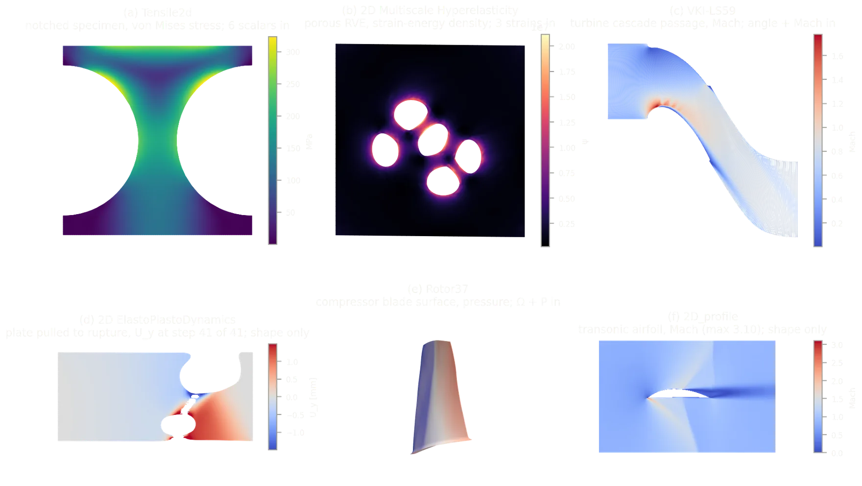
In the PLAID snapshots of 4 September 2026 (7 September for 2D_profile), DIM-GP ranks in the top three on all six boards examined and first on three. When the standalone reconstructed-solver entry is excluded, DIM-GP ranks first on four boards. The excluded entry is the PhysicsX simulator on Tensile2d [44]. The comparison field includes NPco from NP Company and PXTransolver from PhysicsX.
On LagrangeBench, which evaluates particle-based, time-evolving physical systems, DIM-GP improves on the best of three published baselines in 19 of 21 dataset–metric comparisons. The baselines include Google DeepMind’s Graph Network-based Simulator (GNS) [34]. This result extends the evidence beyond mesh-based surrogate models to Lagrangian dynamics.
On AhmedML and DrivAerML, DIM-GP has the lowest reported errors among the ten methods listed, including Emmi AI’s AB-UPT [40], across all five AhmedML channels and both DrivAerML surface channels.
On DeformingPlate, DIM-GP achieves 57% lower RMSE than Google DeepMind’s MeshGraphNets [48] and ranks second among the three methods compared under the canonical protocol (§9).
In our reconstruction of the TabArena-Lite comparison, DIM-GP ranks third among 80 model entries, or sixth among 85 entries including AutoML systems, in an internal comparison using published results (§4). The field includes TabPFN-3 from Prior Labs, acquired by SAP in July 2026. On TALENT-300, it has the lowest average rank in each task type when added to TALENT’s published comparison tables. In a virtual concrete-formulation study based on public laboratory data, STOCHOS meets the modeled specification in 149 of 150 runs, compared with 137 for BoTorch’s qNEHVI.
The scorecard
Bold type highlights DIM-GP results and selected summary findings. Error metrics are lower-is-better unless otherwise stated.
Swipe or scroll horizontally to view all columns →
| Benchmark | DIM-GP result | Field | Interpretation |
|---|---|---|---|
| PLAID VKI-LS59 (§13) | 1st | 21 entries | 7.9% lower aggregate error than PXTransolver. |
| PLAID Hyperelasticity (§14) | 1st | 22 entries | Approximately 6% lower aggregate error than PXTransolver. |
| PLAID ElastoPlastoDynamics (§16) | 1st | 8 entries | Lowest errors on both displacement channels. |
| PLAID Tensile2d (§15) | 2nd | 22 entries | Second overall at an aggregate error of 0.0007. |
| PLAID Rotor37 (§12) | 3rd | 16 entries | Aggregate error approximately 0.00049 versus 0.00043 for the leader: a gap of about 0.00006. |
| PLAID 2D_profile (§17) | 3rd | 22 entries | Aggregate error 0.0152 versus the leader’s 0.0134: a gap of 0.0018. |
| TabArena-51 (§4) | 3rd (internal) | 80 entries | Internal reconstruction; sixth of 85 with AutoML systems. |
| TALENT-300 (§5) | 1st | 29–32 methods | Lowest average rank in all three published comparison fields. |
| AhmedML (§10) | 1st | 10 methods | Lowest error on all five channels; 6.7 h training. |
| DrivAerML (§11) | 1st | 10 methods | Lowest error on both surface channels; under 15 h training. |
| LagrangeBench (§7) | 19 of 21 cells | 3 baselines | Compared with the per-cell best of three methods. |
| DeepMind Water-3D (§8) | 8.5% higher MSE | GNS | Compared with published GNS mean; fewer gradient updates. |
| DeepMind DeformingPlate (§9) | 2nd | 3 methods | 57% lower RMSE than MeshGraphNets; M4GN reports lower RMSE. |
| Bayesian optimization (§18) | 1st in success count | 6 approaches | Highest success count in the virtual study: 149/150 runs. |
The scorecard counts each tabular suite once, each PLAID board separately, and the other studies individually. DIM-GP records 12 top-three placements across 14 evaluated tasks and studies. It also improves on the best of three published LagrangeBench baselines in 19 of 21 dataset–metric comparisons. Across the 12 ranked comparisons, DIM-GP finishes ahead of more than 200 benchmark entries. This count is comparison-specific: a method appearing in several benchmarks contributes one entry to each comparison.
PLAID positions use the archived 4 September 2026 snapshots, except for 2D_profile, which uses the 7 September snapshot. Automotive results are reported as of 7 September 2026.
A transient benchmark example
This animation shows a held-out PLAID 2D ElastoPlastoDynamics test design (§16), comparing the reference simulation with DIM-GP's predicted 41-step transient response.
Computational requirements
One DrivAerML reference simulation requires approximately 61,000 CPU core-hours according to the dataset’s reported setup (§11). Once reference data are available, a trained surrogate can evaluate additional geometries at substantially lower computational cost. Figure 1 reports the training resources for the automotive comparisons.
Scope of the comparisons
The comparison includes named research methods and submissions from commercial vendors. On the five PLAID boards with entries from all three, DIM-GP has lower aggregate error than PXTransolver and NPco on VKI-LS59, Hyperelasticity and Tensile2d, and higher error on Rotor37 and 2D_profile. The separate PhysicsX simulator entry is reported in §15 [44].
1. STOCHOS in the engineering workflow
1.1 What DIM-GP is
DIM-GP stands for Deep Infinite Mixture of Gaussian Processes, the probabilistic model family within STOCHOS. It supports predictions from tables, particle states and unstructured meshes. An engineer can use these models to estimate a material property, predict an aerodynamic field or model a transient response, with uncertainty estimates accompanying the predictions.
The tabular evaluation uses a fixed configuration across the 51 TabArena and 300 TALENT datasets, including validation-based adaptation. Physics evaluations use task-appropriate configurations. The benchmark sections report the results of these configured workflows.
1.2 Incorporating physics into DIM-GP
DIM-GP can incorporate inexpensive physical priors, post-training conditioning on known relationships, and geometric or physical features that help it learn from engineering data. STOCHOS calculates supported geometric features automatically during mesh processing; engineers can supply application-specific physical priors and constraints. Multi-fidelity modeling also allows lower-cost simulations and higher-fidelity simulations or measurements to contribute to the same modeling workflow.
1.3 From models to engineering decisions
STOCHOS Flow connects data import, model fitting, validation, sensitivity analysis and optimization in a visual workflow. Sensitivity analysis identifies influential inputs; Bayesian optimization uses predictions and uncertainty to propose the next design or experiment. Engineers can connect Ansys Workbench or Python solvers and export prediction applications for colleagues to use. Agentic AI assists with workflow creation and troubleshooting, with local model options available.
The benchmark series evaluates the prediction and optimization methods that support this workflow.
1.4 How the results are evaluated
PLAID provides externally scored evidence. Participants receive test inputs, such as geometries and operating conditions, and submit prediction files while the reference test outputs remain withheld. The platform scores the predictions and uses hidden test subsets to discourage overfitting (PLAID benchmark protocol, §4.3 and Appendix C). This allows STOCHOS to be evaluated without distributing its proprietary implementation.
The automotive and tabular sections compare our evaluations with published reference results; §4.2 explains the submission requirements behind the internal TabArena comparison. The formulation study uses a virtual test bench based on public laboratory data. Each section identifies its comparison field, metrics and evaluation conditions.
2. Tabular benchmarks and evaluation protocol
Swipe or scroll horizontally to view all columns →
| TabArena-51 | TALENT-300 | |
|---|---|---|
| Datasets | 51 curated, real-world | 300 |
| Protocol | TabArena-Lite (single split, fold 0) | single seed, fixed splits |
| Metrics | roc_auc (30 sets), log_loss (8), rmse (13) | RMSE / accuracy |
| Field | 79 model variants + 5 AutoML systems | 28–31 published methods (official) + 3 foundation models we added |
| Hardware | 1× RTX 4090; DIM-GP <8 GB | same |
Hardware. The experiments used an Intel Core i9-13900KS workstation (24 cores, 32 threads), 64 GB of DDR5-4200 memory and NVIDIA GeForce RTX 4090 graphics under Windows 11 Pro. The workstation contains two cards, used for separate experiments; each DIM-GP run uses at most one GPU, with GPU memory below 8 GB. Published baseline timings identify their own hardware.
Our TabArena comparison uses fold 0 under the official TabArena-Lite protocol and the corresponding published Lite results. TALENT uses its fixed splits.
2.0 Definitions
Let be the set of methods, the set of datasets, and the error of method on dataset under that dataset’s own metric — one minus ROC-AUC on the 30 binary sets, log-loss on the 8 multiclass sets, RMSE on the 13 regression sets. Lower is better throughout. Because these three quantities share no scale, no statistic below averages across datasets directly.
Elo. TabArena fits a Bradley–Terry model [29] to pairwise wins across datasets. The model assigns method a probability of beating method :
Reported Elo is the median over 200 task-level bootstrap rounds, with confidence bounds at the 2.5% and 97.5% quantiles. Elo reflects who wins; normalized error also reflects the size of error differences. Section 4.2 reports both, together with mean rank.
Normalized error. Per dataset, the error is rescaled against the best and the median method on that dataset, then clipped:
Here, denotes the best observed method and the median or a worse result. Clipping limits the influence of a single unusually large error on the aggregate.
Headroom (§2.1) measures how much a dataset separates methods at all, using the same two quantities as that denominator:
means the median error approaches the best observed error. Larger values indicate greater separation between the best and median.
Cost. Training and inference costs normalize the complete fit and prediction pass by the number of rows, then take the median across datasets:
These measures include fixed per-dataset overhead. Section 4.5 estimates fixed and per-row contributions with a robust Theil–Sen fit [30], .
2.1 What is in TabArena-51
TabArena contains 51 curated real-world datasets [1], checked for leakage, duplication and mislabelled task types. Each dataset has a fixed evaluation metric (Figure 3).
Swipe or scroll horizontally to view all columns →
| Task | Datasets | Metric | Rows (median) | Rows (range) | Features (median) |
|---|---|---|---|---|---|
| Binary | 30 | roc_auc | 9,911 | 748 – 150,000 | 21 |
| Multiclass | 8 | log_loss | 2,445 | 898 – 78,053 | 37 |
| Regression | 13 | rmse | 6,497 | 907 – 53,940 | 9 |
The suite spans 748 to 150,000 rows and 4 to 1,776 features. Binary classification accounts for 30 of the 51 datasets and uses ROC-AUC, a measure of predicted ordering.
Where the data comes from, and how hard it is
TabArena covers commercial and scientific applications; business, marketing and finance account for nearly half the datasets. Figure 4 and the table below summarize their domains and the median-to-best error gaps defined in §2.0.
Swipe or scroll horizontally to view all columns →
| Field | Datasets | Training rows | Median headroom |
|---|---|---|---|
| Business & marketing | 16 | 1,000 – 86,586 | 12.3 % |
| Finance | 8 | 666 – 100,000 | 5.8 % |
| Chemistry & material science | 6 | 598 – 30,486 | 10.5 % |
| Medical & healthcare | 6 | 498 – 47,678 | 10.5 % |
| Biology & life sciences | 5 | 604 – 2,500 | 15.0 % |
| Technology & internet | 4 | 902 – 7,256 | 15.3 % |
| Physics & astronomy | 3 | 1,002 – 52,035 | 24.9 % |
| Industry & manufacturing | 1 | 50,666 | 51.9 % |
| Environmental science & climate | 1 | 1,722 | 9.1 % |
| Education | 1 | 2,949 | 6.9 % |
The suite includes imbalanced industrial and credit tasks, as well as categorical inputs. These characteristics make the stated metric and consistent preprocessing important to the comparison.
2.2 What is in TALENT-300
TALENT provides 300 datasets [2]: 119 regression, 101 binary and 80 multiclass, spanning 252 to 634,460 rows (median 3,389) and 3 to 970 features (median 16), across 15 application domains — finance and economics (53 datasets), healthcare (31), image and signal (28), industrial and sensors (27), biology and genomics (21), and others.
TabArena emphasizes curated comparisons against an actively maintained field. TALENT extends the evaluation across more datasets and application domains.
3. Tabular model families and competitive context
3.1 The three families in the field
The comparison includes three established families: gradient-boosted trees, neural networks trained per dataset and pretrained tabular models.
Gradient-boosted decision trees — LightGBM [18], CatBoost [19] and XGBoost [20] — are widely used tabular methods that fit per dataset and support CPU execution. The comparison includes both default and tuned configurations.
Neural networks for tabular data include RealMLP [21], TabM [22], ModernNCA [23] and xRFM [24]. RealMLP uses defaults developed across multiple datasets and is the highest-ranked non-pretrained entry in this comparison, at tenth place.
Tabular foundation models learn across tasks before adapting to a new dataset. The field includes TabPFN [5, 6] and its variants, TabICL [7], TabFM [3], EXAONE-Tabular [4], TabDPT [9], LimiX [8], Mitra [10] and other published models [11–17]. TabFM and EXAONE-Tabular lead the TabArena comparison presented here.
3.2 Parameter counts and interpretation
The released configurations illustrate the range of model sizes: TabFM [3] contains 1,639,444,298 parameters (1.64 billion) and EXAONE-Tabular [4] contains 20,807,434. DIM-GP is fitted to each dataset and its parameterization varies with the task, so it does not have one fixed parameter count that can be placed fairly beside those foundation models. Section 4 therefore compares measured benchmark performance and computational requirements.
4. TabArena-51
DIM-GP ranks third among 80 model entries by Elo, mean rank and normalized error in our internal reconstruction of TabArena-Lite. Including AutoML systems places it sixth among 85 entries. The following sections describe the scoring check, comparison field and computational cost.
Hover for each entry's score and training time. The amber point is DIM-GP in the internal comparison of §4; hardware differences are discussed in §4.5.
4.1 Scoring validation
Our comparison was rebuilt from TabArena’s published per-method results and compared against the official splits_lite CSVs:
Swipe or scroll horizontally to view all columns →
| Method | official (lite) | ours | Δ |
|---|---|---|---|
| TabFM+ | 1836 | 1840.9 | +4.9 |
| AutoGluon 1.6 (noncommercial) | 1831 | 1832.5 | +1.5 |
| TabFM (default) | 1796 | 1799.8 | +3.8 |
| AutoGluon 1.6 (extreme) | 1757 | 1757.9 | +0.9 |
| EXAONE-Tabular (default) | 1746 | 1744.7 | −1.3 |
| AutoGluon 1.5 (extreme) | 1646 | 1645.1 | −0.9 |
| TabPFN-3 (default) | 1639 | 1638.5 | −0.5 |
| TabPFN-2.6 (default) | 1604 | 1603.2 | −0.8 |
| TabICLv2 (default) | 1555 | 1555.7 | +0.7 |
The selected reference ratings are reproduced within 4.9 Elo points. The official comparison data were obtained from the leaderboard Space’s published results.
4.2 Standing — internal
Comparison status. TabArena’s submission protocol requires executable training and evaluation code integrated into its benchmark. STOCHOS is licensed commercial software and was not provided through that integration route. Its results are therefore reported as an internal comparison with TabArena’s published results.
Selected positions from the models field (AutoML systems excluded):
Swipe or scroll horizontally to view all columns →
| # | Model | Overall | Class. | Regr. | Binary | Multi. | Small | Medium |
|---|---|---|---|---|---|---|---|---|
| 1 | TabFM | 1793 | 1752 | 2168 | 1780 | 1699 | 1785 | 1911 |
| 2 | EXAONE-Tabular | 1749 | 1747 | 1919 | 1756 | 1752 | 1698 | 2021 |
| 3 | DIM-GP | 1652 | 1635 | 1861 | 1654 | 1606 | 1649 | 1751 |
| 4 | TabPFN-3 | 1644 | 1617 | 1897 | 1634 | 1594 | 1624 | 1789 |
| 5 | TabPFN-2.6 | 1613 | 1590 | 1847 | 1585 | 1645 | 1596 | 1747 |
| 6 | RealTabPFN-2.5 (t+e) | 1600 | 1573 | 1849 | 1547 | 1745 | 1595 | 1700 |
| 7 | TabICLv2 | 1555 | 1554 | 1696 | 1573 | 1520 | 1536 | 1691 |
| 10 | RealMLP (t+e) | 1490 | 1475 | 1666 | 1489 | 1451 | 1476 | 1608 |
| 16 | CatBoost (tuned) | 1391 | 1388 | 1494 | 1378 | 1457 | 1354 | 1561 |
All entries are (default) configurations unless marked (t+e) = tuned + ensembled. Rows 1–7 are foundation models, 10 a neural network, 16 tree-based.
With systems included, DIM-GP is 6th of 85 at 1647, just above AutoGluon 1.5 extreme (1646) and TabPFN-3 (1639); AutoGluon 1.6 (1757/1831) and TabFM+ (1836) rank above.
Agreement across ranking measures
Mean rank averages each method’s position across datasets; normalized error also reflects the size of error differences (§2.0). Both give DIM-GP the same placement as Elo:
Swipe or scroll horizontally to view all columns →
| # | Model | Elo | Mean rank | Normalized error | Win rate |
|---|---|---|---|---|---|
| 1 | TabFM | 1793 | 6.18 | 0.1860 | 0.934 |
| 2 | EXAONE-Tabular | 1749 | 7.66 | 0.2501 | 0.916 |
| 3 | DIM-GP | 1652 | 11.27 | 0.3902 | 0.870 |
| 4 | TabPFN-3 | 1644 | 11.66 | 0.3909 | 0.865 |
| 5 | TabPFN-2.6 | 1613 | 13.18 | 0.4384 | 0.846 |
| 6 | RealTabPFN-2.5 (t+e) | 1600 | 13.83 | 0.4483 | 0.838 |
| 7 | TabICLv2 | 1555 | 16.24 | 0.4728 | 0.807 |
DIM-GP is third under all three measures, with the same ordering of the top nine entries. The margin to TabPFN-3 is small: approximately eight Elo points and normalized errors of 0.3902 versus 0.3909. The paired analysis below assesses the differences across datasets.
Split by task type, the picture matches §4.3:
Swipe or scroll horizontally to view all columns →
| Place | Normalized error | Directly ahead | |
|---|---|---|---|
| Classification (38 datasets) | 3 of 78 | 0.4234 | EXAONE 0.2543 |
| Regression, rmse (13 datasets) | 5 of 77 | 0.3256 | TabPFN-3 0.2966, Nori-30M 0.3183 |
Against TabPFN-3, DIM-GP has lower normalized error on classification (0.4234 versus 0.4334) and higher error on regression. TabArena contains 13 regression datasets; the complementary TALENT comparison covers 116 (§5.2).
Statistical comparisons
The paired analysis compares methods on the same 51 datasets using a Wilcoxon signed-rank test [31] on normalized-error differences and an exact sign test on wins and losses. Negative differences favour DIM-GP.
Swipe or scroll horizontally to view all columns →
| Rival | W–L | Mean Δ | Wilcoxon | Sign | Conclusion |
|---|---|---|---|---|---|
| LightGBM (tuned + ens.) | 44–7 | −0.353 | <0.001 | <0.001 | DIM-GP better |
| CatBoost (tuned + ens.) | 39–12 | −0.338 | <0.001 | 0.0002 | DIM-GP better |
| LimiX | 40–10 | −0.283 | <0.001 | <0.001 | DIM-GP better |
| TabICLv2 | 30–20 | −0.076 | 0.059 | 0.203 | no significant difference detected |
| TabPFN-2.6 | 32–19 | −0.045 | 0.124 | 0.092 | no significant difference detected |
| TabPFN-3 | 27–23 | +0.001 | 0.730 | 0.672 | not distinguishable |
| EXAONE-Tabular | 22–29 | +0.140 | 0.011 | 0.401 | mixed |
| TabFM | 9–41 | +0.204 | <0.001 | <0.001 | TabFM better |
A Friedman test over thirteen leading methods rejects equal performance ( , ). The Nemenyi post-hoc comparison [32] uses a critical distance of 2.56 average-rank points at (Figure 8).
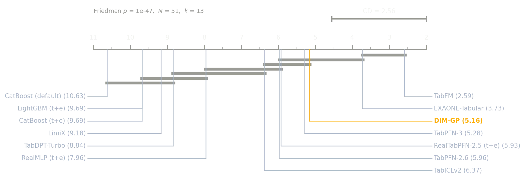
Within this thirteen-method comparison, DIM-GP’s average rank is 5.16 and only TabFM is significantly ahead of DIM-GP under the Nemenyi analysis. RealMLP, TabDPT-Turbo, LimiX and both tuned tree ensembles are significantly behind. Neither paired test detects a significant difference between DIM-GP and TabPFN-3.
Pairwise p-values are unadjusted across the eight comparisons; the Nemenyi procedure controls its thirteen-method comparison. EXAONE-Tabular differs under the unadjusted Wilcoxon test but falls within the Nemenyi critical distance. The paired table and model-only aggregate table use different normalization pools, so their mean-error differences are computed separately.
4.3 Per-axis reading
Selected task-wise comparisons against TabPFN-3:
Swipe or scroll horizontally to view all columns →
| Axis | DIM-GP | TabPFN-3 | Δ |
|---|---|---|---|
| Classification | 1635 | 1617 | +18 |
| Binary | 1654 | 1634 | +20 |
| Small datasets | 1649 | 1624 | +25 |
| Multiclass | 1606 | 1594 | +12 |
| Regression | 1861 | 1897 | −36 |
| Medium datasets | 1751 | 1789 | −38 |
DIM-GP has higher Elo on four of the six reported axes and lower Elo on regression and medium-sized datasets in these descriptive subgroup comparisons.
4.4 Which field DIM-GP is compared in
TabArena distinguishes individual models from AutoML systems that manage model selection and training budgets. The evaluated DIM-GP configuration is fixed across datasets. Section 4.2 reports its placement in both comparison fields.
4.5 Computational cost and hardware
Using TabArena’s cost definition (§2.0), DIM-GP records median times of 30.26 seconds per 1,000 training rows and 2.509 seconds per 1,000 prediction rows on the RTX 4090 (51 datasets, fold 0), placing 32nd of 80 by reported fit cost. The robust timing fit separates fixed per-dataset and per-row contributions:
Swipe or scroll horizontally to view all columns →
| Fixed cost / dataset | Per 1,000 rows | Median s/1K | measured on | |
|---|---|---|---|---|
| TabICLv2 | 5.7 s | 0.42 s | 1.96 | official board |
| TabPFN-3 | 14.2 s | 0.71 s | 3.59 | official board |
| EXAONE-Tabular | 8.3 s | 2.43 s | 6.17 | official board |
| DIM-GP | 10.5 s | 17.74 s | 30.26 | our RTX 4090 |
| TabFM | 33.6 s | 26.00 s | 40.79 | official board |
These fits describe complete training or conditioning procedures. Baseline timings come from the published leaderboard; DIM-GP timings are measured on our RTX 4090.
Hardware sensitivity. The official benchmark records H200 timings for TabPFN-3, TabICLv2, TabPFN-2.6 and LimiX; RTX PRO 6000 timings for TabFM and TabDPT-Turbo; and A100 timings for TabPFN-Wide. To examine the effect of hardware, we ran TabICLv2 through the official harness on our RTX 4090, using the same data splits, preprocessing and eight-fold bagging configuration:
Swipe or scroll horizontally to view all columns →
| Dataset | Rows | fit, RTX 4090 | fit, H200 | Factor |
|---|---|---|---|---|
| blood-transfusion-service-center | 499 | 4.33 s | 4.39 s | 0.99 |
| diabetes | 512 | 4.33 s | 4.09 s | 1.06 |
| qsar-biodeg | 705 | 5.66 s | 5.47 s | 1.03 |
| churn | 3,400 | 6.24 s | 5.65 s | 1.10 |
| bank-marketing | 45,211 | 27.39 s | 13.26 s | 2.07 |
| Bioresponse | 3,751 | 173.92 s | 70.21 s | 2.48 |
| APSFailure | 76,000 | 298.29 s | 107.18 s | 2.78 |
The RTX 4090-to-H200 fit-time ratio ranges from 0.99 to 2.78 across these datasets, showing that hardware effects depend on the workload.
Applying the fitted size-dependent factor to DIM-GP gives an illustrative H200-equivalent estimate of 21.02 s/1K, versus 30.26 s/1K measured on our RTX 4090. This is not a measured DIM-GP H200 run; transferring a calibration from another model adds uncertainty.
The official entries use eight-fold bagging, while DIM-GP uses a single fit. The cost comparison reports these configurations on the shared tasks and split.
Full TabArena-51 board, 80 entries (click to expand; every column sorts; ¹ DIM-GP times are our own measurement on an RTX 4090, section 4.5)
Swipe or scroll horizontally to view all columns →
| # | model | Type | Elo | fit s/1k | infer s/1k | Class. | Regr. | Binary | Multi. | Small | Medium |
|---|---|---|---|---|---|---|---|---|---|---|---|
| 1 | TabFM (default) | Foundation Model | 1793.0 | 40.79 | 6.991 | 1752.0 | 2168.0 | 1780.0 | 1699.0 | 1785.0 | 1911.0 |
| 2 | EXAONE-Tabular (default) | Foundation Model | 1749.0 | 6.17 | 0.623 | 1747.0 | 1919.0 | 1756.0 | 1752.0 | 1698.0 | 2021.0 |
| 3 | DIM-GP | Foundation Model | 1651.5 | 30.26¹ | 2.509¹ | 1635.4 | 1860.9 | 1654.0 | 1606.1 | 1649.0 | 1751.0 |
| 4 | TabPFN-3 (default) | Foundation Model | 1644.0 | 3.59 | 0.395 | 1617.0 | 1897.0 | 1634.0 | 1594.0 | 1624.0 | 1789.0 |
| 5 | TabPFN-2.6 (default) | Foundation Model | 1613.0 | 5.75 | 0.6 | 1590.0 | 1847.0 | 1585.0 | 1645.0 | 1596.0 | 1747.0 |
| 6 | RealTabPFN-2.5 (tuned + ensembled) | Foundation Model | 1600.0 | 2059.94 | 9.785 | 1573.0 | 1849.0 | 1547.0 | 1745.0 | 1595.0 | 1700.0 |
| 7 | TabICLv2 (default) | Foundation Model | 1555.0 | 1.96 | 0.146 | 1554.0 | 1696.0 | 1573.0 | 1520.0 | 1536.0 | 1691.0 |
| 8 | RealTabPFN-2.5 (tuned) | Foundation Model | 1547.0 | 2059.94 | 1.03 | 1535.0 | 1727.0 | 1516.0 | 1661.0 | 1538.0 | 1654.0 |
| 9 | RealTabPFN-2.5 (default) | Foundation Model | 1523.0 | 5.72 | 0.611 | 1531.0 | 1626.0 | 1536.0 | 1542.0 | 1562.0 | 1513.0 |
| 10 | RealMLP (tuned + ensembled) | Neural Network | 1490.0 | 2791.97 | 13.886 | 1475.0 | 1666.0 | 1489.0 | 1451.0 | 1476.0 | 1608.0 |
| 11 | TabDPT (tuned + ensembled) | Foundation Model | 1423.0 | 6155.04 | 386.158 | 1367.0 | 1786.0 | 1369.0 | 1388.0 | 1433.0 | 1459.0 |
| 12 | RealMLP (tuned) | Neural Network | 1416.0 | 2791.97 | 0.373 | 1409.0 | 1539.0 | 1418.0 | 1404.0 | 1407.0 | 1510.0 |
| 13 | TabDPT-Turbo (default) | Foundation Model | 1413.0 | 2.02 | 0.183 | 1383.0 | 1638.0 | 1392.0 | 1377.0 | 1416.0 | 1468.0 |
| 14 | TabM (tuned + ensembled) | Neural Network | 1401.0 | 2462.02 | 1.988 | 1404.0 | 1491.0 | 1408.0 | 1414.0 | 1373.0 | 1547.0 |
| 15 | LightGBM (tuned + ensembled) | Tree-based | 1396.0 | 416.63 | 2.236 | 1381.0 | 1542.0 | 1376.0 | 1433.0 | 1359.0 | 1570.0 |
| 16 | CatBoost (tuned) | Tree-based | 1391.0 | 1347.32 | 0.037 | 1388.0 | 1494.0 | 1378.0 | 1457.0 | 1354.0 | 1561.0 |
| 17 | iLTM (tuned + ensembled) | Foundation Model | 1389.0 | 12741.09 | 397.882 | 1388.0 | 1481.0 | 1408.0 | 1337.0 | 1363.0 | 1524.0 |
| 18 | CatBoost (tuned + ensembled) | Tree-based | 1388.0 | 1347.32 | 0.364 | 1381.0 | 1505.0 | 1370.0 | 1457.0 | 1349.0 | 1570.0 |
| 19 | TabDPT (tuned) | Foundation Model | 1377.0 | 6155.04 | 39.452 | 1321.0 | 1731.0 | 1329.0 | 1317.0 | 1391.0 | 1400.0 |
| 20 | ChimeraBoost (tuned + ensembled) | Tree-based | 1367.0 | 518.46 | 0.522 | 1370.0 | 1440.0 | 1394.0 | 1308.0 | 1304.0 | 1630.0 |
| 21 | ModernNCA (tuned + ensembled) | Neural Network | 1365.0 | 4618.5 | 7.735 | 1334.0 | 1582.0 | 1341.0 | 1335.0 | 1297.0 | 1649.0 |
| 22 | TabM (tuned) | Neural Network | 1364.0 | 2462.02 | 0.231 | 1365.0 | 1448.0 | 1361.0 | 1409.0 | 1343.0 | 1482.0 |
| 23 | LimiX (default) | Foundation Model | 1356.0 | 27.33 | 6.11 | 1393.0 | 1314.0 | 1375.0 | 1503.0 | 1400.0 | 1289.0 |
| 24 | XGBoost (tuned + ensembled) | Tree-based | 1355.0 | 700.96 | 1.438 | 1359.0 | 1417.0 | 1362.0 | 1372.0 | 1312.0 | 1539.0 |
| 25 | ChimeraBoost (tuned) | Tree-based | 1344.0 | 518.46 | 0.045 | 1361.0 | 1363.0 | 1381.0 | 1311.0 | 1286.0 | 1579.0 |
| 26 | LightGBM (tuned) | Tree-based | 1341.0 | 416.63 | 0.381 | 1332.0 | 1451.0 | 1316.0 | 1426.0 | 1300.0 | 1518.0 |
| 27 | CatBoost (default) | Tree-based | 1340.0 | 5.81 | 0.025 | 1348.0 | 1390.0 | 1370.0 | 1291.0 | 1296.0 | 1525.0 |
| 28 | ModernNCA (tuned) | Neural Network | 1337.0 | 4618.5 | 0.47 | 1349.0 | 1376.0 | 1363.0 | 1321.0 | 1288.0 | 1540.0 |
| 29 | XGBoost (tuned) | Tree-based | 1332.0 | 700.96 | 0.213 | 1330.0 | 1414.0 | 1328.0 | 1368.0 | 1296.0 | 1491.0 |
| 30 | TabSwift (default) | Foundation Model | 1332.0 | 1.19 | 0.07 | 1319.0 | 1474.0 | 1354.0 | 1205.0 | 1338.0 | 1371.0 |
| 31 | xRFM (tuned + ensembled) | Other | 1328.0 | 866.12 | 2.007 | 1304.0 | 1495.0 | 1296.0 | 1363.0 | 1315.0 | 1414.0 |
| 32 | TabPFNv2 (tuned + ensembled) [35.29% IMPUTED] | Foundation Model | 1312.0 | 2943.39 | 17.365 | – | – | – | – | – | – |
| 33 | iLTM (tuned) | Foundation Model | 1294.0 | 12741.09 | 60.101 | 1300.0 | 1339.0 | 1313.0 | 1269.0 | 1278.0 | 1386.0 |
| 34 | Mitra (default) [35.29% IMPUTED] | Foundation Model | 1292.0 | 87.36 | 2.432 | – | – | – | – | – | – |
| 35 | ChimeraBoost (default) | Tree-based | 1285.0 | 2.54 | 0.05 | 1302.0 | 1293.0 | 1319.0 | 1261.0 | 1223.0 | 1518.0 |
| 36 | xRFM (tuned) | Other | 1282.0 | 866.12 | 0.097 | 1258.0 | 1444.0 | 1257.0 | 1284.0 | 1264.0 | 1381.0 |
| 37 | TabDPT (default) | Foundation Model | 1278.0 | 45.42 | 39.405 | 1214.0 | 1620.0 | 1221.0 | 1202.0 | 1295.0 | 1274.0 |
| 38 | TabM (default) | Neural Network | 1274.0 | 7.81 | 0.237 | 1288.0 | 1287.0 | 1290.0 | 1305.0 | 1266.0 | 1340.0 |
| 39 | TabICL (default) [29.41% IMPUTED] | Foundation Model | 1273.0 | 6.86 | 1.52 | – | – | – | – | – | – |
| 40 | EBM (tuned + ensembled) | Tree-based | 1255.0 | 1877.68 | 0.14 | 1299.0 | 1168.0 | 1301.0 | 1316.0 | 1252.0 | 1310.0 |
| 41 | TabPFNv2 (tuned) [35.29% IMPUTED] | Foundation Model | 1252.0 | 2943.39 | 0.262 | – | – | – | – | – | – |
| 42 | TorchMLP (tuned + ensembled) | Neural Network | 1250.0 | 2832.93 | 1.801 | 1266.0 | 1253.0 | 1275.0 | 1250.0 | 1230.0 | 1343.0 |
| 43 | RealMLP (default) | Neural Network | 1243.0 | 10.44 | 1.714 | 1257.0 | 1253.0 | 1293.0 | 1130.0 | 1246.0 | 1272.0 |
| 44 | SAP-RPT-OSS (default) | Foundation Model | 1239.0 | 13.96 | 2.081 | 1249.0 | 1272.0 | 1239.0 | 1310.0 | 1278.0 | 1163.0 |
| 45 | BetaTabPFN (default) [25.49% IMPUTED] | Foundation Model | 1236.0 | 203.0 | 1.155 | – | – | – | – | – | – |
| 46 | TabPFNv2 (default) [35.29% IMPUTED] | Foundation Model | 1221.0 | 3.27 | 0.315 | – | – | – | – | – | – |
| 47 | ModernNCA (default) | Neural Network | 1217.0 | 13.74 | 0.316 | 1180.0 | 1398.0 | 1201.0 | 1111.0 | 1206.0 | 1276.0 |
| 48 | EBM (tuned) | Tree-based | 1207.0 | 1877.68 | 0.014 | 1245.0 | 1122.0 | 1248.0 | 1253.0 | 1217.0 | 1214.0 |
| 49 | ExtraTrees (tuned + ensembled) | Tree-based | 1197.0 | 257.64 | 0.846 | 1191.0 | 1253.0 | 1167.0 | 1304.0 | 1195.0 | 1225.0 |
| 50 | EBM (default) | Tree-based | 1188.0 | 6.9 | 0.015 | 1242.0 | 1024.0 | 1250.0 | 1230.0 | 1194.0 | 1201.0 |
| 51 | TorchMLP (tuned) | Neural Network | 1187.0 | 2832.93 | 0.112 | 1199.0 | 1204.0 | 1200.0 | 1214.0 | 1181.0 | 1232.0 |
| 52 | XGBoost (default) | Tree-based | 1184.0 | 2.06 | 0.122 | 1200.0 | 1167.0 | 1204.0 | 1204.0 | 1128.0 | 1370.0 |
| 53 | FastaiMLP (tuned + ensembled) | Neural Network | 1169.0 | 594.95 | 4.649 | 1210.0 | 1048.0 | 1215.0 | 1207.0 | 1179.0 | 1170.0 |
| 54 | ExtraTrees (tuned) | Tree-based | 1168.0 | 257.64 | 0.068 | 1159.0 | 1225.0 | 1144.0 | 1234.0 | 1169.0 | 1178.0 |
| 55 | Nori-30M (default) [74.51% IMPUTED] | Foundation Model | 1164.0 | 0.53 | 0.077 | – | – | – | – | – | – |
| 56 | RandomForest (tuned + ensembled) | Tree-based | 1161.0 | 377.14 | 0.747 | 1167.0 | 1158.0 | 1140.0 | 1288.0 | 1141.0 | 1238.0 |
| 57 | Nori (default) [74.51% IMPUTED] | Foundation Model | 1156.0 | 0.53 | 0.077 | – | – | – | – | – | – |
| 58 | LightGBM (default) | Tree-based | 1154.0 | 2.2 | 0.171 | 1150.0 | 1200.0 | 1141.0 | 1201.0 | 1134.0 | 1228.0 |
| 59 | RandomForest (tuned) | Tree-based | 1124.0 | 377.14 | 0.091 | 1130.0 | 1117.0 | 1109.0 | 1224.0 | 1098.0 | 1206.0 |
| 60 | FastaiMLP (tuned) | Neural Network | 1104.0 | 594.95 | 0.336 | 1134.0 | 1014.0 | 1143.0 | 1109.0 | 1127.0 | 1053.0 |
| 61 | PerpetualBooster (tuned + ensembled) | Tree-based | 1082.0 | 176.26 | 0.499 | 1060.0 | 1177.0 | 1106.0 | 817.0 | 1091.0 | 1060.0 |
| 62 | iLTM (default) | Foundation Model | 1080.0 | 301.0 | 65.827 | 1135.0 | 860.0 | 1163.0 | 1019.0 | 1058.0 | 1156.0 |
| 63 | TabSTAR (tuned) | Foundation Model | 1075.0 | 39935.25 | 4.288 | 1115.0 | 939.0 | 1143.0 | 1000.0 | 1115.0 | 958.0 |
| 64 | TabSTAR (tuned + ensembled) | Foundation Model | 1072.0 | 39935.25 | 20.166 | 1105.0 | 976.0 | 1133.0 | 988.0 | 1114.0 | 950.0 |
| 65 | OrionMSP (default) [25.49% IMPUTED] | Foundation Model | 1050.0 | 12.4 | 2.558 | – | – | – | – | – | – |
| 66 | TorchMLP (default) | Neural Network | 1040.0 | 8.96 | 0.129 | 1045.0 | 1024.0 | 1052.0 | 1019.0 | 1023.0 | 1087.0 |
| 67 | PerpetualBooster (tuned) | Tree-based | 1036.0 | 176.26 | 0.191 | 1009.0 | 1133.0 | 1057.0 | 740.0 | 1049.0 | 998.0 |
| 68 | xRFM (default) | Other | 1030.0 | 3.14 | 0.741 | 978.0 | 1203.0 | 939.0 | 1111.0 | 1043.0 | 1006.0 |
| 69 | ExtraTrees (default) | Tree-based | 1007.0 | 1.97 | 0.251 | 987.0 | 1074.0 | 997.0 | 942.0 | 1036.0 | 929.0 |
| 70 | RandomForest (default) | Tree-based | 1000.0 | 0.43 | 0.053 | 1000.0 | 1000.0 | 1000.0 | 1000.0 | 1000.0 | 1000.0 |
| 71 | TabFlex (default) [25.49% IMPUTED] | Foundation Model | 982.0 | 0.8 | 0.119 | – | – | – | – | – | – |
| 72 | FastaiMLP (default) | Neural Network | 979.0 | 3.12 | 0.312 | 1003.0 | 881.0 | 1021.0 | 926.0 | 988.0 | 962.0 |
| 73 | TabSTAR (default) | Foundation Model | 976.0 | 398.79 | 4.645 | 1018.0 | 789.0 | 1059.0 | 808.0 | 1019.0 | 827.0 |
| 74 | KNN (tuned + ensembled) | Baseline | 970.0 | 129.17 | 1.627 | 1000.0 | 854.0 | 995.0 | 1021.0 | 968.0 | 972.0 |
| 75 | PerpetualBooster (default) | Tree-based | 940.0 | 22.76 | 0.025 | 933.0 | 952.0 | 978.0 | 672.0 | 962.0 | 876.0 |
| 76 | Linear (tuned + ensembled) | Baseline | 903.0 | 240.78 | 0.308 | 968.0 | 468.0 | 981.0 | 912.0 | 899.0 | 907.0 |
| 77 | Linear (tuned) | Baseline | 880.0 | 240.78 | 0.068 | 946.0 | 409.0 | 958.0 | 890.0 | 880.0 | 871.0 |
| 78 | KNN (tuned) | Baseline | 822.0 | 129.17 | 0.103 | 842.0 | 722.0 | 846.0 | 805.0 | 820.0 | 807.0 |
| 79 | Linear (default) | Baseline | 821.0 | 1.23 | 0.115 | 887.0 | 271.0 | 919.0 | 718.0 | 837.0 | 757.0 |
| 80 | KNN (default) | Baseline | 606.0 | 0.19 | 0.037 | 566.0 | 625.0 | 612.0 | 214.0 | 623.0 | 559.0 |
5. TALENT-300
We add DIM-GP to TALENT’s published method comparisons for regression, binary classification and multiclass classification.
5.1 Comparison with TALENT’s published methods
TALENT publishes results for 28 regression methods and 31 classification methods, including XGBoost, CatBoost, LightGBM, TabPFN, TabR, ModernNCA and RealMLP.
Swipe or scroll horizontally to view all columns →
| Task | DIM-GP avg rank | field | runner-up |
|---|---|---|---|
| Regression | 2.30 — 1st of 29 | 90 datasets | CatBoost 6.74 |
| Binary | 4.14 — 1st of 32 | 95 datasets | TabR 9.14 |
| Multiclass | 3.00 — 1st of 32 | 77 datasets | RealMLP 6.89 |
DIM-GP has the lowest average rank in each task type within this published comparison field.
5.2 Running on one consumer GPU
DIM-GP completed all 300 datasets on one RTX 4090 while limited to less than 8 GB of GPU memory.
5.3 Protocol
The DIM-GP evaluation uses a single seed and fixed splits; TALENT’s published tables average multiple seeds. Classification is scored by accuracy and regression by RMSE. Average ranks permit comparison across datasets with different target scales.
6. Beyond tabular data: physics surrogates
The physics evaluation covers particle dynamics, contact and large deformation, aerodynamic fields and transient structural response.
6.1 What is being evaluated
Two members of the STOCHOS model family are evaluated:
- DIM-GP Particle — predicts the evolution of particle and mesh-node states (§§7–9).
- DIM-GP — the surrogate for fields on unstructured meshes, evaluated in §§10–17.
6.2 Why these particular benchmarks
The benchmarks cover the following physical regimes and comparison fields:
Swipe or scroll horizontally to view all columns →
| Benchmark | Regime | Comparison field |
|---|---|---|
| LagrangeBench (§7) | Lagrangian SPH dynamics, 7 datasets | GNS, SEGNN, CoRGI |
| DeepMind Water-3D (§8) | Lagrangian, long-horizon rollout | GNS |
| DeepMind DeformingPlate (§9) | Quasi-static solid contact, tetrahedral mesh, 400 steps | MeshGraphNets and M4GN — canonical protocol |
| AhmedML (§10) | Steady 3D automotive aerodynamics | AB-UPT and eight other published methods |
| DrivAerML (§11) | Steady 3D automotive aerodynamics, high fidelity | AB-UPT and eight other published methods |
| PLAID Rotor37 (§12) | Parametric 3D compressor CFD | Public leaderboard |
| PLAID VKI-LS59 (§13) | 2D transonic turbine cascade, RANS | Public leaderboard |
| PLAID 2D Multiscale Hyperelasticity (§14) | Finite-strain RVEs, variable topology | Public leaderboard |
| PLAID Tensile2d (§15) | 2D elastoplastic specimen, parametric | Public leaderboard |
| PLAID 2D ElastoPlastoDynamics (§16) | Transient plate rupture, 41 steps | Public leaderboard |
| PLAID 2D_profile (§17) | Transonic airfoils, shape-only input | Public leaderboard |
PLAID sections report the archived board state of 4 September 2026, except for 2D_profile, which uses the 7 September snapshot. Submissions from commercial vendors are identified by their entry names, so each comparison refers to a specific submission in that snapshot.
![Figure 10. Reference data from four physics benchmarks. Top row: (a) dam break, (b) lid-driven cavity and (c) Taylor–Green vortex from LagrangeBench [33], followed by (d) DeepMind Water-3D [34]. Particle colours show per-step displacement; 3D cutaways expose the interior. Bottom row: (e) AhmedML [39], coloured by static pressure coefficient, and (f) PLAID Rotor37 [41], coloured by surface pressure.](/science/benchmarks/figures/fig9_usecases.webp)
7. LagrangeBench — verified against the benchmark’s own evaluator
LagrangeBench [33] is a Lagrangian-simulation benchmark: seven SPH datasets (2D and 3D Taylor–Green vortex, reverse Poiseuille flow, lid-driven cavity, and 2D dam break), a fixed protocol, and published baselines. It supports comparison across three published methods: GNS [34], SEGNN [35] and CoRGI [36] all publish numbers on the same cells under the same rules.
7.1 Protocol
Scoring follows the benchmark exactly: 26-frame windows made of 6 seed frames and 20 predicted steps, with RPF-2D scored over 384 and RPF-3D over 192 test windows. Three metrics per dataset — MSE20 (position error over the 20 predicted steps, per dimension), Sinkhorn (a distributional divergence, blind to particle identity) and Ekin (squared error of total kinetic energy).
7.2 Result — lower error in 19 of 21 comparisons
Each DIM-GP result is compared with the lowest published error for that dataset and metric across GNS, SEGNN and CoRGI.
Swipe or scroll horizontally to view all columns →
| dataset | metric | best published (holder) | DIM-GP | comparison |
|---|---|---|---|---|
| DAM-2D | MSE20 | 1.55e-5 (CoRGI) | 3.49e-7 | 44× lower error |
| DAM-2D | Sinkhorn | 2.82e-6 (CoRGI) | 6.48e-8 | 44× lower error |
| DAM-2D | Ekin | 2.18e-5 (CoRGI) | 8.88e-8 | 245× lower error |
| LDC-2D | MSE20 | 1.4e-5 (GNS) | 9.34e-6 | 1.50× lower error |
| LDC-2D | Sinkhorn | 5.07e-7 (CoRGI) | 1.15e-7 | 4.39× lower error |
| LDC-2D | Ekin | 3.81e-7 (CoRGI) | 2.76e-7 | 1.38× lower error |
| RPF-2D | MSE20 | 1.54e-6 (CoRGI) | 1.226e-6 | 1.26× lower error |
| RPF-2D | Sinkhorn | 2.08e-8 (CoRGI) | 1.49e-9 | 14× lower error |
| RPF-2D | Ekin | 2.39e-6 (CoRGI) | 7.224e-6 | 3.02× higher error |
| TGV-2D | MSE20 | 3.81e-6 (CoRGI) | 2.29e-6 | 1.67× lower error |
| TGV-2D | Sinkhorn | 1.05e-7 (CoRGI) | 3.56e-8 | 2.95× lower error |
| TGV-2D | Ekin | 2.90e-7 (CoRGI) | 1.35e-7 | 2.15× lower error |
| LDC-3D | MSE20 | 3.86e-5 (CoRGI) | 2.44e-5 | 1.58× lower error |
| LDC-3D | Sinkhorn | 2.64e-7 (CoRGI/SEGNN) | 1.48e-7 | 1.79× lower error |
| LDC-3D | Ekin | 1.55e-8 (CoRGI) | 1.48e-8 | 1.05× lower error |
| RPF-3D | MSE20 | 1.64e-5 (SEGNN) | 1.330e-5 | 1.23× lower error |
| RPF-3D | Sinkhorn | 1.33e-7 (CoRGI) | 6.41e-8 | 2.08× lower error |
| RPF-3D | Ekin | 1.34e-6 (SEGNN) | 1.263e-6 | parity |
| TGV-3D | MSE20 | 5.2e-3 (SEGNN) | 4.76e-3 | 1.10× lower error |
| TGV-3D | Sinkhorn | 6.4e-6 (SEGNN) | 3.07e-6 | 2.09× lower error |
| TGV-3D | Ekin | 2.21e-3 (CoRGI/SEGNN) | 1.86e-3 | 1.19× lower error |
Compared with each method individually, DIM-GP has lower error than GNS on all 21 cells, lower error than SEGNN on 20 with one parity, and lower error than CoRGI on 19.
DIM-GP has the lowest error on all three metrics for DAM-2D, LDC-2D, TGV-2D, LDC-3D and TGV-3D.
Under the Neural-SPH 400-step protocol [37] on DAM-2D, evaluated over all 25 trajectories, the corresponding values are 3.12e-2 / 4.90e-4 / 1.99e-4 against a published best of 8.4e-2 / 7.5e-3 / 2.1e-3, a factor of 2.7 / 15 / 10.6. Since the 20-step protocol is comparatively short, this establishes that the margin persists at twenty times the horizon.
7.3 The remaining two comparisons
RPF-3D Ekin — parity. DIM-GP records 1.263e-6 against SEGNN’s 1.34e-6 and is reported as parity.
RPF-2D Ekin — higher error than CoRGI. DIM-GP has 3.9-fold lower error than GNS and 2.5-fold lower error than SEGNN on this cell, while CoRGI reports the lowest error.
7.4 Cost
Each reported model was trained on a single RTX 4090, at roughly 20–90 seconds per epoch depending on dataset and resolution.
Ground truth against the DIM-GP rollout
Dam break 2D
Lid-driven cavity 2D
Reverse Poiseuille flow 2D
Taylor–Green vortex 2D
Lid-driven cavity 3D
Reverse Poiseuille flow 3D
Taylor–Green vortex 3D
8. DeepMind Water-3D — measured against the published GNS result
Water-3D is the 3D fluid dataset from Learning to Simulate Complex Physics with Graph Networks [34]: approximately 14,000 particles over 800 timesteps. It tests prediction over a much longer rollout than the 20-step LagrangeBench evaluation.
8.1 Result
Scored under the paper’s own protocol — 100 test sequences, full 800-step rollouts, seed frames excluded:
Swipe or scroll horizontally to view all columns →
| model | rollout MSE (mean) | median | thickness | speed | MMD | gradient updates |
|---|---|---|---|---|---|---|
| GNS, as published [34] | 0.01010 | — | — | — | — | ~20M |
| DIM-GP, accuracy setting | 0.01096 | 0.00984 | 82% | 87% | 0.00265 | ~1.9M (10% of GNS) |
| DIM-GP, physics setting | 0.01238 | 0.01109 | 90% | 106% | 0.00249 | ~1.6M |
The accuracy setting has a mean rollout MSE 8.5% above the published GNS value, with approximately one tenth as many gradient updates. The update count describes the training schedule; wall-clock time also depends on the cost of each update.
The second setting improves the physical diagnostics, reaching 90% of reference fluid-column thickness and 106% of characteristic speed, compared with 82% and 87% for the accuracy setting. The two configurations illustrate the choice between minimizing position error and preserving bulk fluid behaviour.
8.2 Comparison scope
The comparison uses the published GNS result on Water-3D under the full 800-step protocol. LagrangeBench reports a different quantity, MSE over 20 predicted steps, while NeuralMPM [38] reports full-rollout results on 2D fluid datasets. Those results belong to their respective datasets and protocols and are evaluated separately from Water-3D.
Ground truth against the DIM-GP rollout
Water-3D
9. DeepMind DeformingPlate — comparison under the canonical protocol
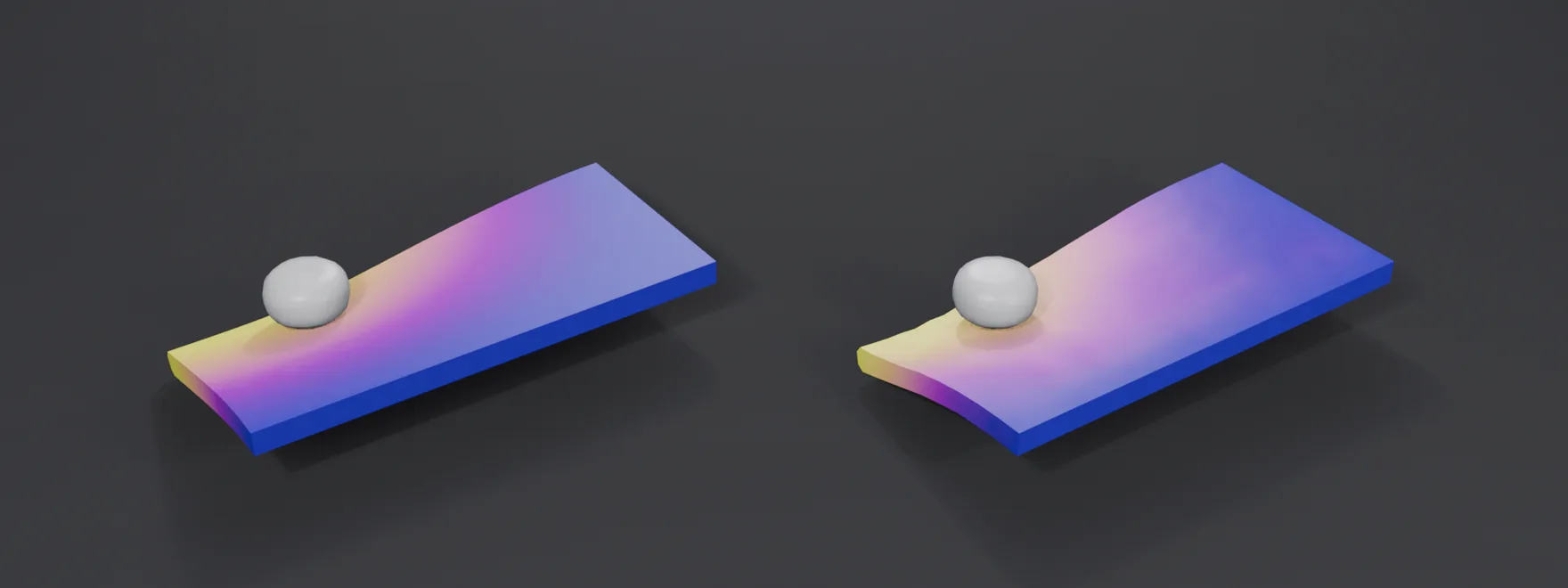
DeformingPlate is the solid-mechanics case of the MeshGraphNets suite [48]: a rigid actuator with a prescribed motion is pressed into a hyperelastic plate that is clamped along one edge, and the plate’s node positions are to be predicted over 400 quasi-static steps on a tetrahedral mesh of 700–2,200 nodes. The task includes contact and large deformation, and every trajectory has its own plate geometry, actuator shape and path. 1,200 trajectories are used for training, 100 for validation and 100 for the test score.
9.1 Protocol
The score follows the original paper: RMSE of world positions in metres over all nodes and all 399 predicted steps of the 100 test trajectories, with errors pooled before taking the square root and reported . The seed frame is excluded. The checkpoint was selected on the validation split, and the test split was scored once.
9.2 Result
Swipe or scroll horizontally to view all columns →
| method | RMSE-all | data and protocol |
|---|---|---|
| canonical: DeepMind data, official split, original error formula | ||
| MeshGraphNets [48] | 15.1 | original paper |
| DIM-GP | 6.45 | this work, checkpoint chosen on the validation split |
| M4GN [49] | 2.65 | reported; no code released, not reproduced |
| not on the canonical protocol, listed for completeness | ||
| MGN-T [50] | 3.21 | data regenerated with COMSOL |
| HCMT [51] | 7.3 | different error formula; its own MeshGraphNets baseline reads 7.8, DIM-GP reads 4.9 under it |
| ROBIN [52] | 4.98 | square root before the mean over trajectories; its own MeshGraphNets baseline reads 8.8 |
| EvoMesh [53] | 12.9 | trained on 500 of the 1,200 trajectories |
| BSMS-GNN [54] | 16.0 | dataset re-split 1000/200/200 |
DIM-GP reports RMSE of 6.45 versus 15.1 for MeshGraphNets, a 57% reduction, and ranks second among the three canonical-protocol entries. M4GN reports the lowest value, 2.65. The remaining rows use different data, splits or error conventions and are listed separately.
9.3 Cost
Training completed in less than one day on a single RTX 4090, with peak GPU memory below 8 GB.
Ground truth against the DIM-GP rollout
Actuator pressing a hyperelastic plate
10. AhmedML — internal evaluation against published baselines
AhmedML [39] is a 500-geometry CFD dataset over the Ahmed body, a standard automotive bluff-body. The published comparison in AB-UPT [40] provides the external baseline values used below.
10.1 Protocol and metric
The metric follows that comparison: per design, the Frobenius relative error , averaged over designs, reported as a percentage. Five channels are scored — surface pressure and wall shear stress ; volume velocity , vorticity and total pressure . Evaluation uses raw full-resolution clouds from the 50 test designs in AB-UPT’s published split.
10.2 Result
Swipe or scroll horizontally to view all columns →
| relative L2 (%) | ↓ | ↓ | ↓ | ↓ | ↓ | reported training |
|---|---|---|---|---|---|---|
| DIM-GP [63] | 2.97 | 3.81 | 1.85 | 6.30 | 1.85 | 6.7 h, 8 GB |
| AB-UPT [40] | 3.01 | 3.88 | 1.90 | 6.52 | 1.98 | ~7 h, H100¹ |
| Transformer [55] | 3.41 | 4.03 | 2.09 | 6.76 | 2.16 | — |
| Transolver [56] | 3.45 | 4.00 | 2.05 | 8.22 | 2.16 | — |
| OFormer [57] | 4.12 | 4.60 | 3.63 | 15.06 | 4.08 | — |
| UPT [58] | 4.25 | 5.80 | 2.73 | 15.03 | 3.10 | — |
| Graph U-Net [59] | 6.46 | 7.29 | 4.15 | 53.66 | 5.18 | — |
| GINO [60] | 7.90 | 8.18 | 6.23 | 71.81 | 8.10 | — |
| PointNet [61] | 8.02 | 10.09 | 5.44 | 66.04 | 6.13 | — |
| LNO [62] | 12.95 | 11.50 | 7.59 | 72.49 | 8.48 | — |
AhmedML test geometry run_241 (official test split): surface pressure of the reference simulation and of the DIM-GP prediction, displayed on a decimated surface mesh. Drag to orbit, scroll to zoom, right-drag to pan.
¹ AB-UPT’s paper reports approximately seven hours on one NVIDIA H100 for AhmedML [40].
DIM-GP places first of ten on all five channels in the comparison with published baselines [40]. Relative to AB-UPT, error is lower by 1.3% on surface pressure, 1.8% on wall shear, 2.6% on volume velocity, 3.4% on vorticity and 6.6% on total pressure.
The DIM-GP row reports our internal evaluation as of 7 September 2026. Baseline values come from the published comparison [40]. The ranking is based on point estimates.
10.3 Training time and hardware
DIM-GP trains in 6.7 hours on one RTX 4090 under an 8 GB memory cap. AB-UPT reports approximately seven hours on one NVIDIA H100 for AhmedML [40].
For a same-device estimate, we scale AB-UPT’s published H100 time using NVIDIA’s official peak memory-bandwidth and mixed-precision Tensor-throughput specifications for the H100 PCIe, H100 SXM and RTX 4090 [64–66]. The resulting RTX 4090-equivalent range is approximately 14–42 hours. Against that range, DIM-GP uses approximately 52–84% less training time, corresponding to a 2.1–6.3× time ratio. This is a specification-normalized estimate; realized scaling depends on workload and hardware utilization.
11. DrivAerML — internal evaluation against published baselines
DrivAerML [43] comprises 484 usable variants of the DrivAer notchback vehicle, each solved by hybrid RANS–LES (SA- -DDES, OpenFOAM) on a ~160M-cell mesh at a cost of roughly 40 hours on 1,536 CPU cores per design — on the order of 61,000 core-hours per geometry. The learning task is steady: one geometry in, the time-averaged surface pressure and wall-shear-stress fields out (~8.8M surface cells). Evaluation follows AB-UPT [40]: its published 400/34/50 split and per-design relative L2 error, using the Frobenius norm over the three shear components and averaging over the 50 test designs.
Swipe or scroll horizontally to view all columns →
| relative L2 (%) | surface pressure | wall shear | trained on | reported training |
|---|---|---|---|---|
| DIM-GP [63] | 3.74 | 7.15 | surface only | under 15 h |
| AB-UPT [40] | 3.82 | 7.29 | surface + volume | 6.9 h, H100² |
| Transformer [55] | 4.35 | 8.26 | surface + volume | — |
| Transolver [56] | 4.81 | 8.95 | surface + volume | — |
| OFormer [57] | 4.85 | 8.92 | surface + volume | — |
| UPT [58] | 7.44 | 12.93 | surface + volume | — |
| GINO [60] | 13.03 | 21.71 | surface + volume | — |
| Graph U-Net [59] | 16.13 | 27.84 | surface + volume | — |
| LNO [62] | 20.51 | 36.44 | surface + volume | — |
| PointNet [61] | 23.63 | 41.85 | surface + volume | — |
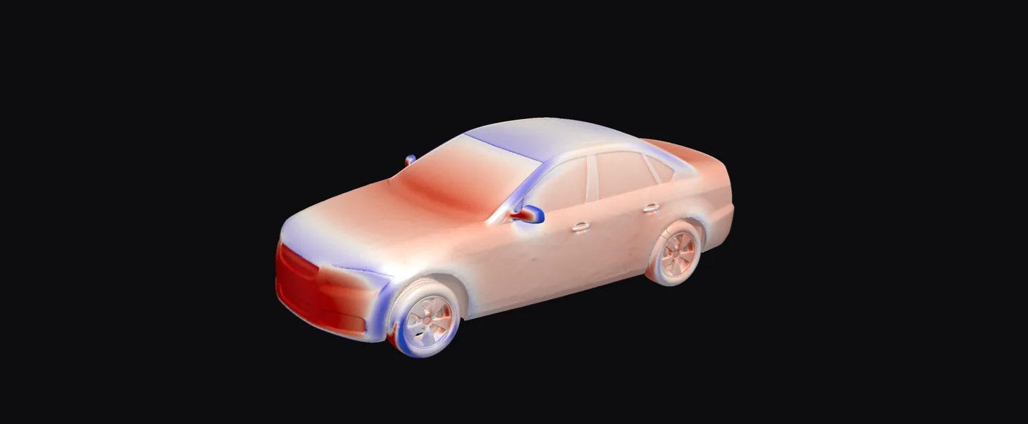
DrivAerML test car run_11: surface pressure of the reference simulation and of the DIM-GP prediction, displayed on a decimated surface mesh. Drag to orbit, scroll to zoom, right-drag to pan.
² Published mixed-FP16 training time for 500 epochs on one NVIDIA H100 [40].
DIM-GP places 1st of 10 on both channels, with 2.1% less surface-pressure error and 1.9% less wall-shear error than runner-up AB-UPT. The DIM-GP values report our internal evaluation as of 7 September 2026. Baseline values come from the published comparison [40]. The ranking is based on point estimates.
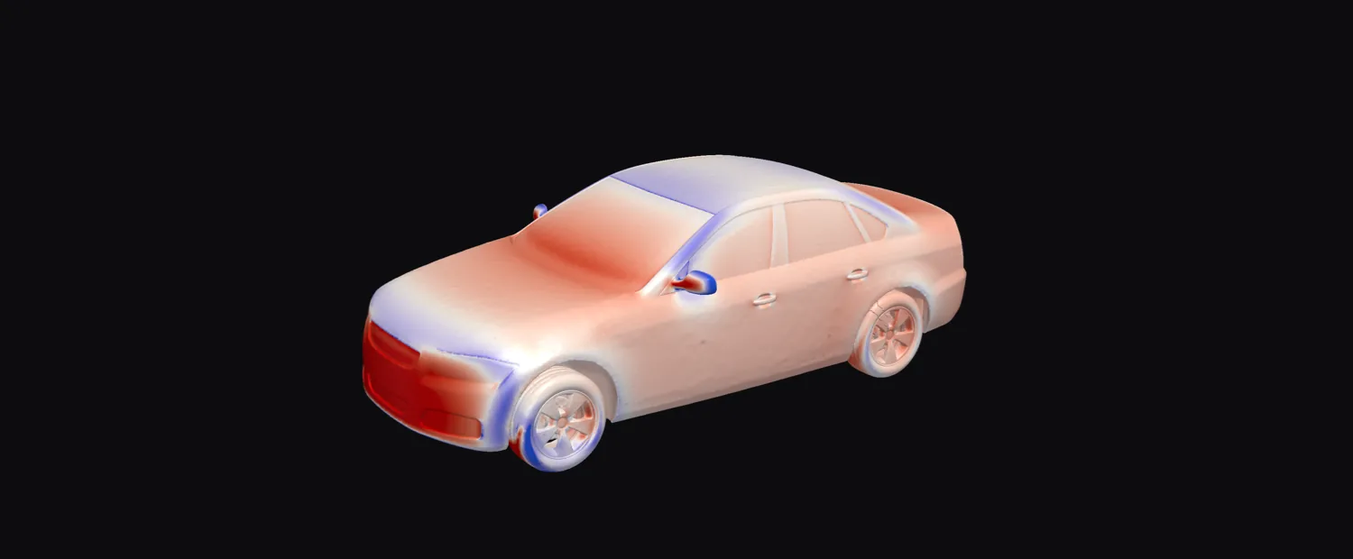 referenceDIM-GP
Drag the slider: reference simulation on the left of the divider, DIM-GP prediction on the right (same colour scale). The three-panel figure below adds the difference map.
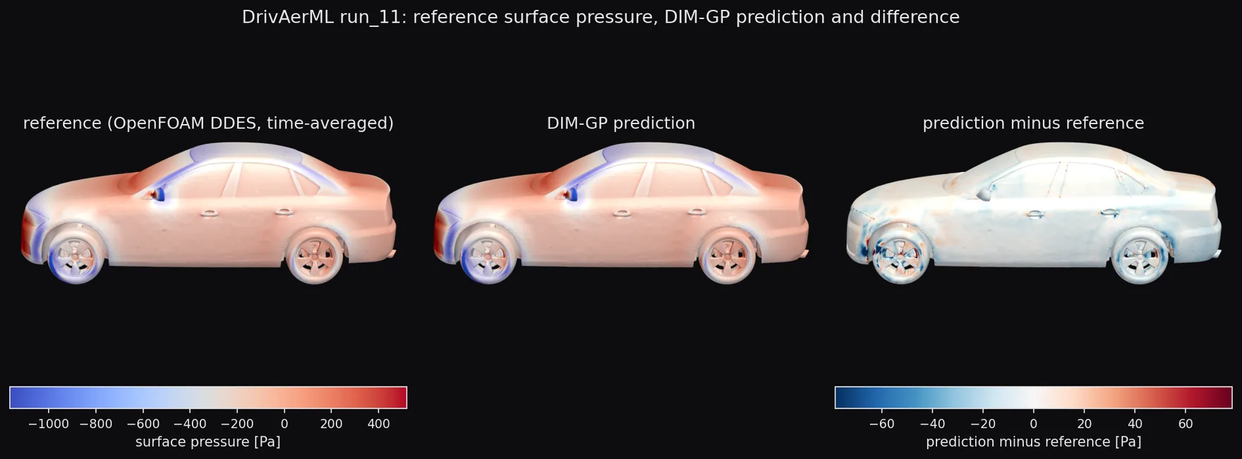
11.1 Training resources
DIM-GP completes surface-only training in under 15 hours on one RTX 4090, with GPU memory limited to less than 8 GB. AB-UPT reports 6.9 hours on one H100 for its mixed-FP16, 500-epoch surface-and-volume configuration, and 33.6 hours for full FP32 [40].
12. PLAID Rotor37 — live leaderboard, third placeboard state as of 4 September 2026
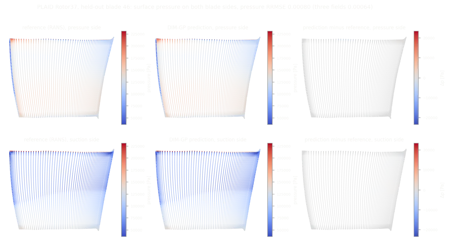
Rotor37 [41] is part of the PLAID benchmark suite (Safran, CC-BY-SA): 1,000 training and 200 test designs of a transonic axial compressor blade, 29,773 surface nodes each, with two operating scalars (rotational speed , inlet pressure ) as input and three surface fields (density, pressure, temperature) plus three global quantities (mass flow, compression ratio, isentropic efficiency) as output. All six are scored by a server-side leaderboard.
In the 4 September 2026 snapshot, DIM-GP ranks 3rd of 16 at a total error of 0.000488 (displayed 0.0005), behind NPco (~0.00043) and PXTransolver (~0.00047) and ahead of Super-MARIO (~0.00077). The gap to NPco is approximately 0.00006 in aggregate RRMSE, or 0.006 percentage points when expressed as percentages (approximately 0.049% versus 0.043%).
Swipe or scroll horizontally to view all columns →
| RRMSE (lower is better) | Density | Pressure | Temp. | Massflow | Compr. ratio | Efficiency | total |
|---|---|---|---|---|---|---|---|
| NPco | 0.0007 | 0.0007 | 0.0003 | 0.0003 | 0.0003 | 0.0003 | 0.0004 |
| PXTransolver | 0.0008 | 0.0008 | 0.0003 | 0.0003 | 0.0003 | 0.0003 | 0.0005 |
| DIM-GP | 0.0008 | 0.0008 | 0.0003 | 0.0003 | 0.0003 | 0.0003 | 0.0005 |
| Super-MARIO | 0.0013 | 0.0013 | 0.0005 | 0.0005 | 0.0005 | 0.0005 | 0.0008 |
| MMGP | 0.0031 | 0.003 | 0.0008 | 0.0005 | 0.0005 | 0.0005 | 0.0014 |
| MeshFiLM | 0.0027 | 0.0027 | 0.0007 | 0.0008 | 0.0009 | 0.0008 | 0.0014 |
| MARIO | 0.0035 | 0.0034 | 0.001 | 0.0008 | 0.0007 | 0.0006 | 0.0017 |
| Baburu | 0.0042 | 0.0042 | 0.0014 | 0.0007 | 0.0007 | 0.0009 | 0.002 |
| Stealth | 0.0029 | 0.0029 | 0.0009 | 0.0027 | 0.0027 | 0.0019 | 0.0023 |
| ICLGS | 0.0047 | 0.0047 | 0.0011 | 0.0021 | 0.0019 | 0.0014 | 0.0026 |
| Vi-Transformer | 0.0063 | 0.0062 | 0.0019 | 0.001 | 0.0011 | 0.0007 | 0.0029 |
| Augur | 0.0055 | 0.0053 | 0.0012 | 0.0028 | 0.0028 | 0.0019 | 0.0033 |
| tp140205 | 0.0139 | 0.0136 | 0.0025 | 0.0047 | 0.0043 | 0.0042 | 0.0072 |
| MGN | 0.0114 | 0.0114 | 0.0024 | 0.0061 | 0.006 | 0.0071 | 0.0074 |
| GeoFunFlow-3D | 0.0319 | 0.0315 | 0.0134 | 0.0376 | 0.0383 | 0.0138 | 0.0278 |
| FNO | 0.084 | 0.0836 | 0.0086 | 0.0046 | 0.0042 | 0.0031 | 0.0313 |
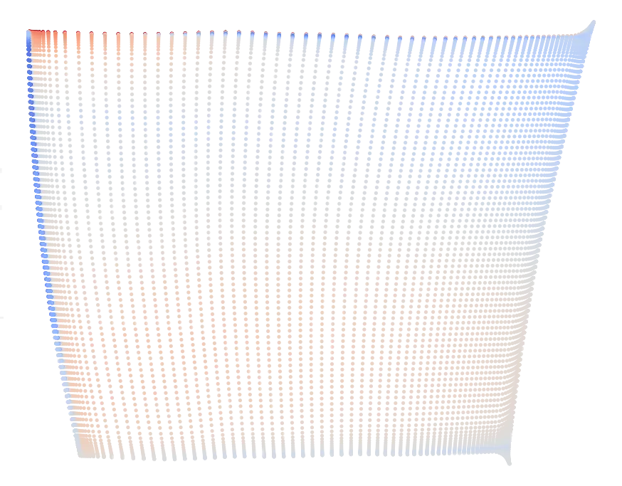
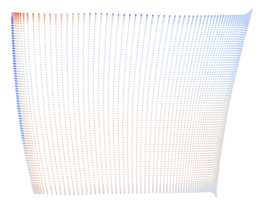 referenceDIM-GP
Drag the slider: reference simulation on the left of the divider, DIM-GP prediction on the right (same colour scale). The three-panel figure below adds the difference map.
13. PLAID VKI-LS59 — live leaderboard, first placeboard state as of 4 September 2026
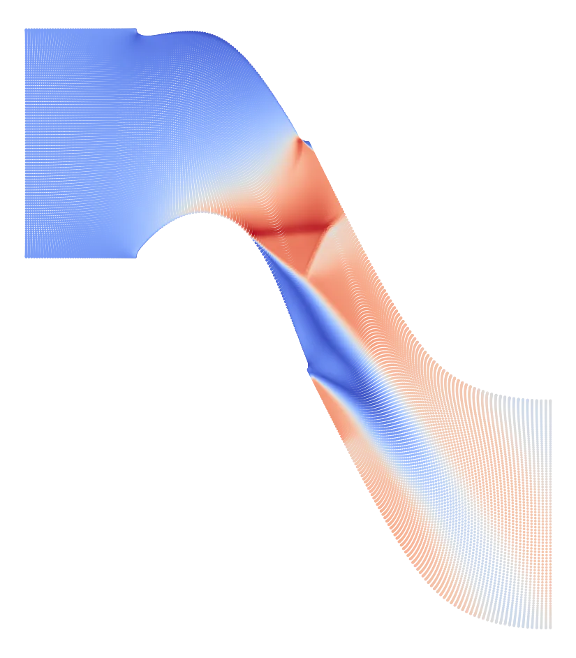
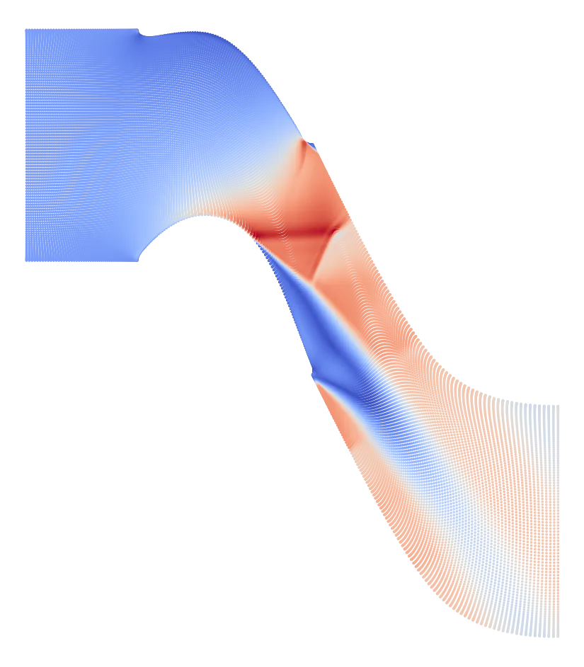
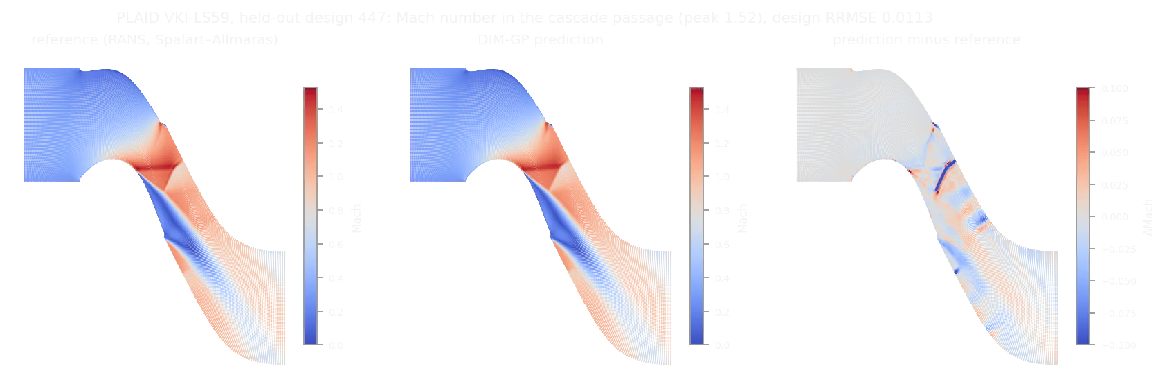
VKI-LS59 [41] is the suite’s 2D transonic turbine cascade: 671 training and 168 test profiles of a linear cascade (Safran, CC-BY-SA), 36,421 nodes each, solved by compressible RANS (Spalart–Allmaras) with the passage reaching Mach 1.78. Inputs are two operating scalars (inlet angle, outlet Mach number) and the mesh; the competition scores two nodal fields (Mach number and turbulent viscosity ) and six global quantities ( , power, the pressure and temperature ratios and , the isentropic efficiency and the outlet angle).
Swipe or scroll horizontally to view all columns →
| RRMSE (lower is better) | nut | mach | Q | power | Pr | Tr | eth_is | angle_out | total |
|---|---|---|---|---|---|---|---|---|---|
| DIM-GP | 0.0216 | 0.0093 | 0.0025 | 0.0062 | 0.0015 | 0 | 0.0306 | 0.0022 | 0.0093 |
| PXTransolver | 0.0205 | 0.0084 | 0.0039 | 0.0044 | 0.0015 | 0 | 0.0402 | 0.0023 | 0.0101 |
| NPco | 0.0243 | 0.0094 | 0.0025 | 0.0067 | 0.0018 | 0 | 0.0433 | 0.0019 | 0.0112 |
| MARIO | 0.0259 | 0.0112 | 0.0052 | 0.0077 | 0.0018 | 0 | 0.0453 | 0.0023 | 0.0124 |
| ICLGS | 0.0344 | 0.0155 | 0.0035 | 0.0092 | 0.0013 | 0 | 0.0375 | 0.0037 | 0.0131 |
| MeshFiLM | 0.0283 | 0.0102 | 0.0077 | 0.0091 | 0.002 | 0 | 0.0486 | 0.0025 | 0.0135 |
| CRT | 0.0337 | 0.0185 | 0.0015 | 0.0053 | 0.0018 | 0 | 0.0466 | 0.0023 | 0.0137 |
| SAIR | 0.0278 | 0.0122 | 0.0015 | 0.0049 | 0.0025 | 0 | 0.0586 | 0.0026 | 0.0138 |
| Stealth | 0.035 | 0.0176 | 0.0029 | 0.0067 | 0.0027 | 0 | 0.0699 | 0.0032 | 0.0173 |
| gantnera | 0.0329 | 0.0131 | 0.0109 | 0.0083 | 0.0026 | 0 | 0.0669 | 0.0037 | 0.0173 |
| Vi-Transformer | 0.0498 | 0.0232 | 0.0052 | 0.0083 | 0.0024 | 0 | 0.0621 | 0.0031 | 0.0193 |
| MARIO (Samy) | 0.0403 | 0.0208 | 0.0054 | 0.008 | 0.0029 | 0 | 0.0898 | 0.0033 | 0.0213 |
| FNO | 0.0846 | 0.018 | 0.0047 | 0.0062 | 0.0019 | 0 | 0.0539 | 0.0027 | 0.0215 |
| test | 0.0412 | 0.0186 | 0.0034 | 0.0052 | 0.0029 | 0 | 0.0976 | 0.0041 | 0.0216 |
| Augur | 0.0424 | 0.0221 | 0.012 | 0.0113 | 0.0027 | 0 | 0.0863 | 0.0045 | 0.0227 |
| Rrrra | 0.0423 | 0.0182 | 0.0189 | 0.0158 | 0.0038 | 0 | 0.0852 | 0.0071 | 0.0239 |
| MMGP+ | 0.0822 | 0.0309 | 0.0023 | 0.0057 | 0.0026 | 0 | 0.1224 | 0.0033 | 0.0312 |
| MGN | 0.0771 | 0.0156 | 0.0716 | 0.0403 | 0.0064 | 0.0001 | 0.1625 | 0.0241 | 0.0497 |
| transolver | 0.0532 | 0.0139 | 1 | 1 | 1 | 1 | 1 | 1 | 0.7584 |
| Naive_approach_GP | 0.0669 | 0.0384 | 1 | 1 | 1 | 1 | 1 | 1 | 0.7632 |
| akabalan_1fieldTesting | 0.2849 | 0.0175 | 1 | 1 | 1 | 1 | 1 | 1 | 0.7878 |
The entry holds first place of 21 at 0.0093, approximately 8% lower aggregate error than PXTransolver. It leads the efficiency column and maintains competitive errors across the other scored outputs.
 referenceDIM-GP
Drag the slider: reference simulation on the left of the divider, DIM-GP prediction on the right (same colour scale). The three-panel figure below adds the difference map.
14. PLAID 2D Multiscale Hyperelasticity — live leaderboard, first placeboard state as of 4 September 2026
This benchmark [41] is the suite’s variable-topology case: 764 training and 376 test representative volume elements of a porous hyperelastic material, each a different microstructure with five to eight holes (constant total porosity, node counts from 4,100 to 7,100), solved by FEniCS at finite strain. Inputs are three macroscopic strain components and the mesh; the competition scores seven nodal fields — the displacements , the four components of the first Piola–Kirchhoff stress, and the strain-energy density — together with the homogenised effective energy. Every design has its own mesh topology.
Swipe or scroll horizontally to view all columns →
| RRMSE (lower is better) | u1 | u2 | P11 | P12 | P22 | P21 | psi | eff. energy | total |
|---|---|---|---|---|---|---|---|---|---|
| DIM-GP | 0.003 | 0.0031 | 0.0093 | 0.0139 | 0.0095 | 0.0136 | 0.0263 | 0.002 | 0.0101 |
| PXTransolver | 0.0026 | 0.0028 | 0.0093 | 0.014 | 0.0095 | 0.0139 | 0.0262 | 0.0074 | 0.0107 |
| test | 0.0065 | 0.0064 | 0.0166 | 0.0256 | 0.017 | 0.0254 | 0.0267 | 0.0042 | 0.0161 |
| NPco | 0.0029 | 0.0028 | 0.0198 | 0.0285 | 0.0202 | 0.0283 | 0.0259 | 0.0037 | 0.0165 |
| plaidtest | 0.0068 | 0.007 | 0.0181 | 0.0278 | 0.0184 | 0.0275 | 0.0292 | 0.0057 | 0.0176 |
| T&D | 0.0059 | 0.0061 | 0.0201 | 0.0298 | 0.0205 | 0.0297 | 0.0266 | 0.0067 | 0.0182 |
| Stealth | 0.0055 | 0.0058 | 0.0231 | 0.033 | 0.0236 | 0.0329 | 0.0264 | 0.0039 | 0.0193 |
| MiSe-GNN | 0.012 | 0.014 | 0.0173 | 0.0312 | 0.0176 | 0.0314 | 0.0328 | 0.0111 | 0.0209 |
| aravabt | 0.006 | 0.0066 | 0.026 | 0.0368 | 0.0263 | 0.0364 | 0.0265 | 0.0055 | 0.0213 |
| Augur | 0.0109 | 0.0114 | 0.0208 | 0.0336 | 0.0212 | 0.033 | 0.0274 | 0.0188 | 0.0221 |
| MeshFiLM | 0.0091 | 0.0097 | 0.0261 | 0.0377 | 0.0267 | 0.0377 | 0.0281 | 0.008 | 0.0229 |
| test | 0.0119 | 0.0167 | 0.0262 | 0.0403 | 0.0267 | 0.0399 | 0.0295 | 0.0231 | 0.0268 |
| FNO | 0.0115 | 0.0117 | 0.0353 | 0.0513 | 0.0359 | 0.051 | 0.0329 | 0.012 | 0.0302 |
| test1 | 0.0132 | 0.014 | 0.0329 | 0.0532 | 0.0326 | 0.0519 | 0.033 | 0.0117 | 0.0303 |
| Vi-Transformer | 0.0173 | 0.0172 | 0.0337 | 0.0581 | 0.0343 | 0.0571 | 0.0312 | 0.0113 | 0.0325 |
| Unet | 0.0291 | 0.0283 | 0.0349 | 0.0498 | 0.0347 | 0.05 | 0.035 | 0.018 | 0.035 |
| Pmh | 0.0161 | 0.0176 | 0.0366 | 0.0643 | 0.0367 | 0.0625 | 0.0362 | 0.0226 | 0.0366 |
| ICLGS | 0.0244 | 0.029 | 0.0473 | 0.0872 | 0.0482 | 0.0864 | 0.0433 | 0.0183 | 0.048 |
| MARIO | 0.0336 | 0.0377 | 0.0536 | 0.1067 | 0.0539 | 0.1053 | 0.0456 | 0.022 | 0.0573 |
| GP | 0.0748 | 0.075 | 0.0809 | 0.167 | 0.0815 | 0.1667 | 0.054 | 0.0216 | 0.0902 |
| MuFi-MiSe | 0.0108 | 0.0132 | 0.0305 | 0.0466 | 0.0307 | 0.0465 | 0.0315 | 1 | 0.1512 |
| transolver | 0.0129 | 0.0121 | 0.0327 | 0.0613 | 0.0332 | 0.0544 | 0.0335 | 1 | 0.155 |
The entry ranks first of 22 at 0.010093 (displayed 0.0101), approximately 6% below PXTransolver in aggregate error. The four stress errors are comparable to PXTransolver’s. DIM-GP has the lowest effective-energy error, 0.0020, followed by NPco at 0.0037 and PXTransolver at 0.0074.
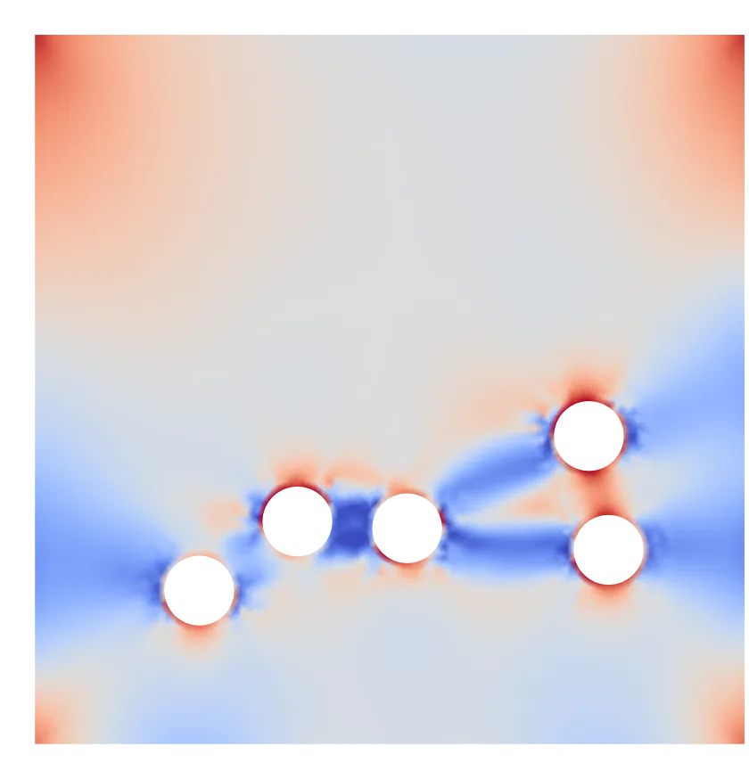
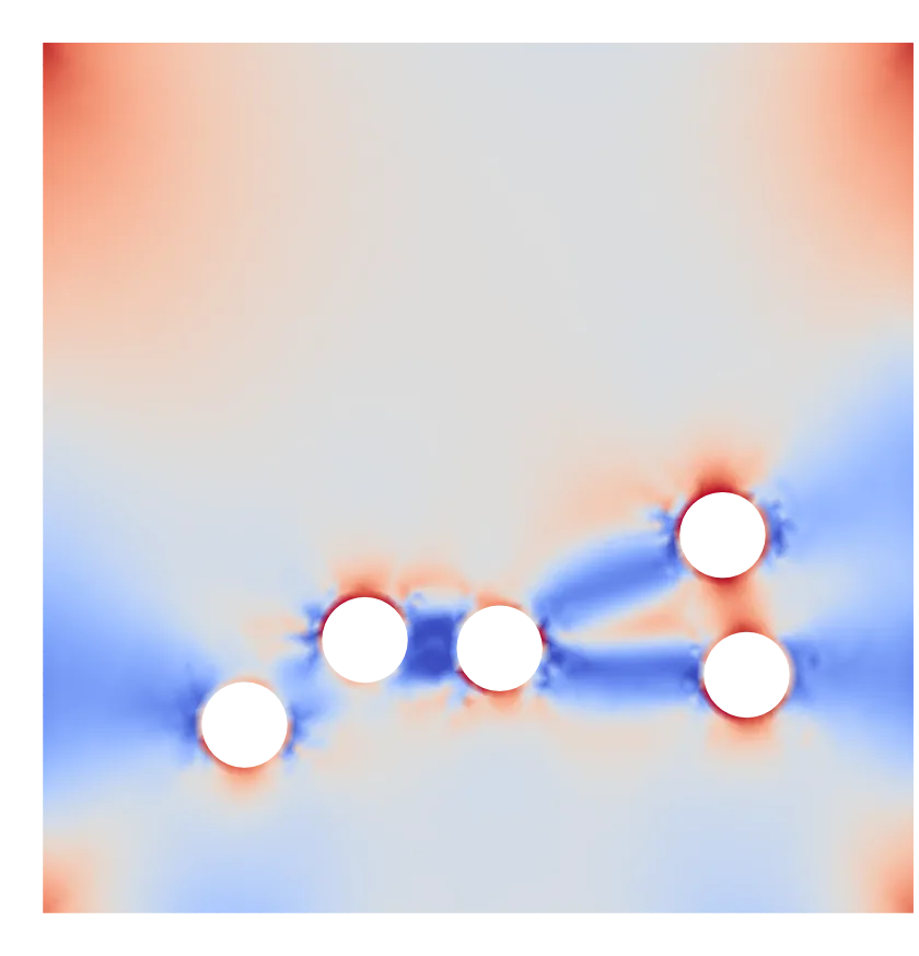 referenceDIM-GP
Drag the slider: reference simulation on the left of the divider, DIM-GP prediction on the right (same colour scale). The three-panel figure below adds the difference map.
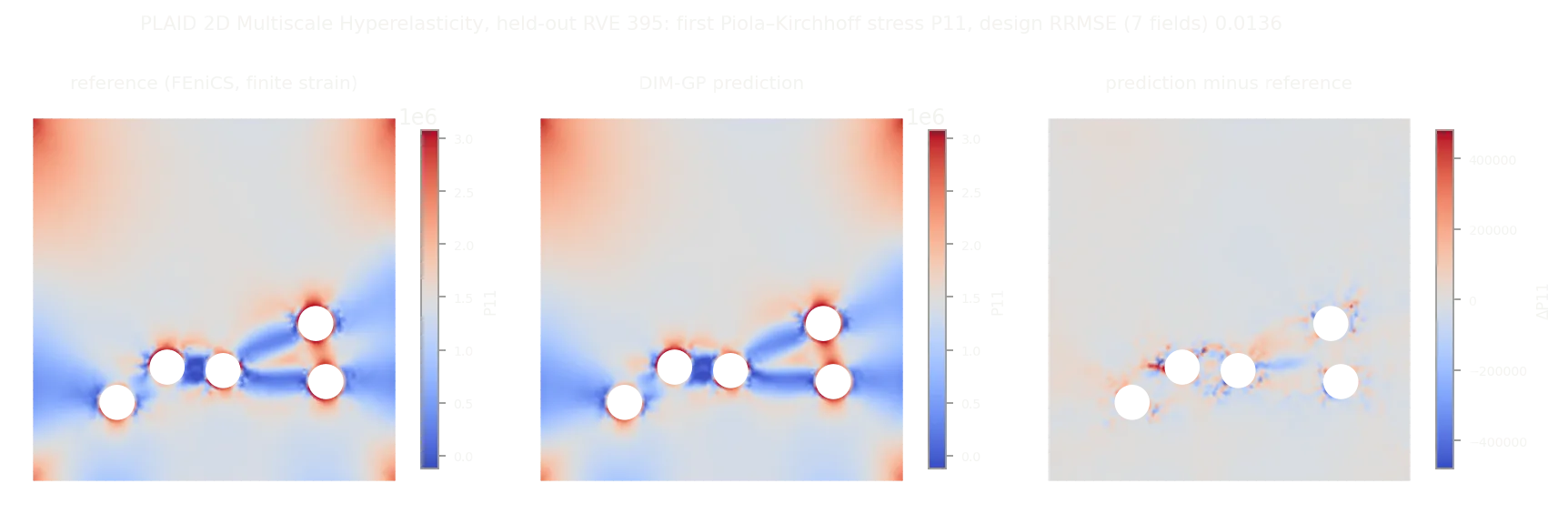
15. PLAID Tensile2d — live leaderboard, second place behind a declared solverboard state as of 4 September 2026
Tensile2d [41] is the suite’s entry-level structural case: a 2D plane-strain, quasi-static, small-strain elastoplastic specimen under a uniform top traction, meshed once per design with 6,000–10,000 nodes (Safran, Z-set solver). Inputs are six scalars — the load , four parameters of the isotropic hardening law and the Young’s modulus — and the mesh; the competition scores five nodal fields ( , , , , ) and three scalars (the maximum von Mises stress, and the maximum and on the top edge). 500 designs carry labels, 200 form the test set.
Swipe or scroll horizontally to view all columns →
| RRMSE (lower is better) | U1 | U2 | sig11 | sig22 | sig12 | max vM | max U2 top | max sig22 top | total |
|---|---|---|---|---|---|---|---|---|---|
| PhysicsX Agent (reverse-engineered) | 0 | 0 | 0 | 0 | 0 | 0 | 0 | 0 | 0 |
| DIM-GP | 0.0004 | 0.0005 | 0.0013 | 0.0006 | 0.0012 | 0.0004 | 0.001 | 0.0004 | 0.0007 |
| NPco | 0.0002 | 0.0003 | 0.0013 | 0.0006 | 0.0009 | 0.0044 | 0.0006 | 0.0016 | 0.0013 |
| PhysicsX Transolver | 0.0002 | 0.0002 | 0.0012 | 0.0006 | 0.0009 | 0.0046 | 0.0008 | 0.0017 | 0.0013 |
| Stealth | 0.0003 | 0.0003 | 0.0012 | 0.0006 | 0.0009 | 0.0048 | 0.0008 | 0.0016 | 0.0013 |
| MeshFiLM | 0.0002 | 0.0003 | 0.0012 | 0.0006 | 0.0009 | 0.005 | 0.0022 | 0.0015 | 0.0015 |
| plaidtest | 0.0013 | 0.0017 | 0.0029 | 0.0013 | 0.0018 | 0.0051 | 0.003 | 0.0017 | 0.0023 |
| PassionTraining | 0.0009 | 0.0011 | 0.0021 | 0.001 | 0.0016 | 0.0066 | 0.0044 | 0.0019 | 0.0025 |
| MMGP | 0.0015 | 0.0009 | 0.0031 | 0.0013 | 0.0021 | 0.005 | 0.0053 | 0.0017 | 0.0026 |
| test | 0.0015 | 0.0022 | 0.0036 | 0.0016 | 0.0024 | 0.0069 | 0.0025 | 0.0019 | 0.0028 |
| ICLGS | 0.0028 | 0.004 | 0.0048 | 0.0018 | 0.0032 | 0.0065 | 0.0021 | 0.0018 | 0.0034 |
| CRT | 0.0013 | 0.0015 | 0.0057 | 0.0022 | 0.0039 | 0.0079 | 0.0024 | 0.0026 | 0.0034 |
| sangmin12312343 | 0.0018 | 0.0018 | 0.003 | 0.0019 | 0.0023 | 0.0108 | 0.0066 | 0.0016 | 0.0037 |
| MARIO | 0.0023 | 0.003 | 0.004 | 0.0017 | 0.0023 | 0.0088 | 0.0063 | 0.0023 | 0.0038 |
| MMVT | 0.0043 | 0.0051 | 0.0089 | 0.0037 | 0.0051 | 0.0068 | 0.0073 | 0.0019 | 0.0054 |
| Augur | 0.0037 | 0.0048 | 0.0081 | 0.0035 | 0.005 | 0.0101 | 0.014 | 0.0034 | 0.0066 |
| MGN | 0.0034 | 0.0043 | 0.0047 | 0.0013 | 0.0016 | 0.0169 | 0.0292 | 0.0022 | 0.008 |
| Vi-Transformer | 0.0086 | 0.0091 | 0.0184 | 0.0102 | 0.0146 | 0.009 | 0.0203 | 0.0021 | 0.0116 |
| FNO | 0.0174 | 0.011 | 0.025 | 0.0057 | 0.0135 | 0.0085 | 0.0152 | 0.0021 | 0.0123 |
| JBone | 0.3054 | 0.3891 | 0.4022 | 0.2354 | 0.268 | 0.0052 | 0.0017 | 0.0017 | 0.2011 |
| MuFi-MiSe | 0.0023 | 0.0036 | 0.0042 | 0.002 | 0.0024 | 1 | 1 | 1 | 0.3768 |
| transolver | 0.0029 | 0.0036 | 0.0049 | 0.0016 | 0.0022 | 1 | 1 | 1 | 0.3769 |
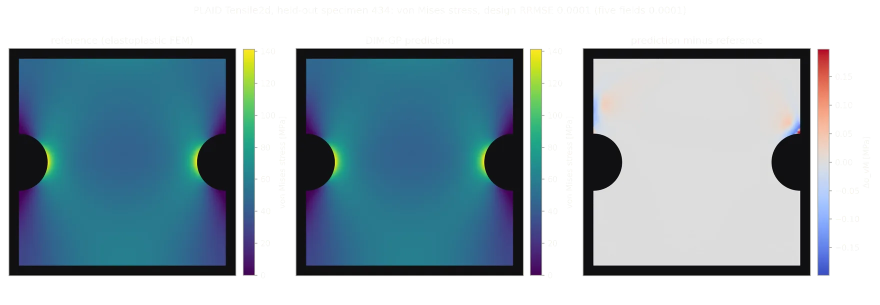
DIM-GP ranks second of 22 at a displayed aggregate error of 0.0007. In its article How an AI Agent Cracked an Industry Benchmark, PhysicsX reports that AI agents reconstructed the reference simulator by inferring the constitutive law and simulation setup from the supplied training data [44]. Its entry ranks first with zero error at the leaderboard’s displayed precision.
The DIM-GP workflow runs on the CPU in minutes.
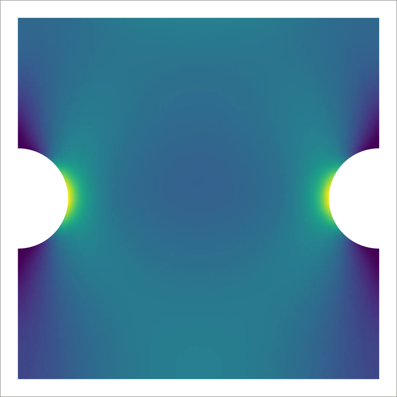
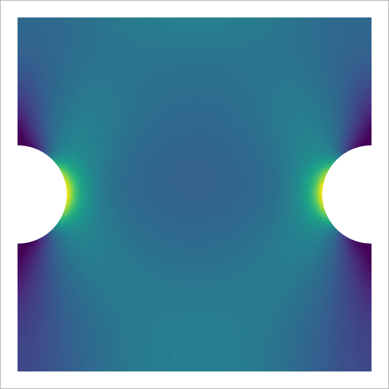 referenceDIM-GP
Drag the slider: reference simulation on the left of the divider, DIM-GP prediction on the right (same colour scale). The three-panel figure below adds the difference map.
16. PLAID 2D ElastoPlastoDynamics — live leaderboard, first placeboard state as of 4 September 2026
This is a transient solid-mechanics case [41]: a 200 × 100 mm steel plate with up to four holes and edge notches, clamped on the left and pulled at 500 mm/s on the right, computed by the benchmark’s authors with an explicit finite-element solver, a non-linear, non-local constitutive law and element erosion, and delivered as 41 time steps of the two displacement fields on 19,000–30,000 nodes per design. There are no input scalars: the geometry is the only variable, 1,000 designs are labelled and 18 form the test set. The competition scores the full and trajectories.
Transient field prediction substantially increases the scale of the learning problem. Each design contains a sequence of complete mesh fields rather than a single steady-state solution. Here, 41 time steps across 19,000–30,000 nodes produce approximately 0.8–1.2 million node-time states per design and output field. Memory use and training cost therefore grow rapidly with both spatial resolution and sequence length, particularly for architectures that represent mesh states as large token sequences. This makes the benchmark a demanding test of an architecture’s ability to model high-resolution spatial fields and their evolution over time.
Swipe or scroll horizontally to view all columns →
| RRMSE (lower is better) | U_x | U_y | total |
|---|---|---|---|
| DIM-GP | 0.0005 | 0.0167 | 0.0086 |
| test | 0.0008 | 0.017 | 0.0089 |
| DAFNO | 0.0025 | 0.0291 | 0.0158 |
| FNO | 0.0031 | 0.0399 | 0.0215 |
| Vi-Transformer | 0.0186 | 0.0269 | 0.0227 |
| MGN | 0.0073 | 0.0403 | 0.0238 |
| MARIO | 0.0059 | 0.058 | 0.0319 |
| Augur | 0.0264 | 0.0427 | 0.0346 |
The entry holds first place of eight at 0.008605, with the lowest displayed and errors in the archived table. The displayed values are 0.0005 for DIM-GP and 0.0008 for the next entry.
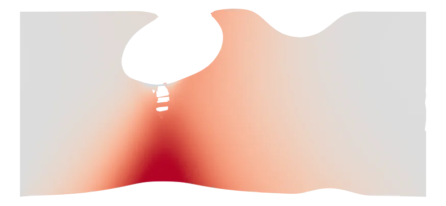
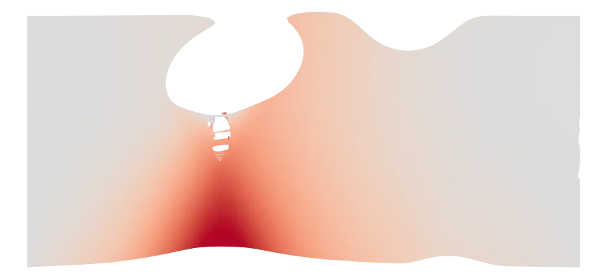 referenceDIM-GP
Drag the slider: reference simulation on the left of the divider, DIM-GP prediction on the right (same colour scale). The three-panel figure below adds the difference map.
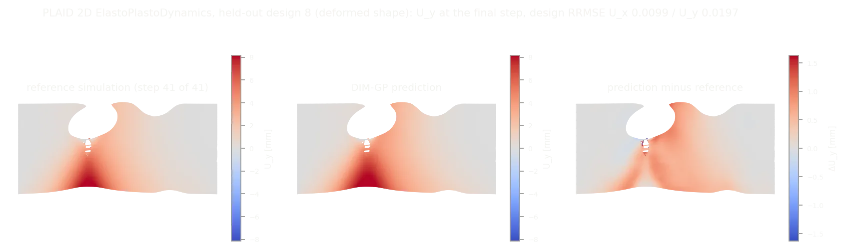
The board metric normalises each field by its maximum over the whole test set, with constants of roughly 340 mm ( ) and 25 mm ( ).
Ground truth against the DIM-GP rollout
Perforated steel plate pulled to rupture
17. PLAID 2D_profile — live leaderboard, third placeboard state as of 7 September 2026
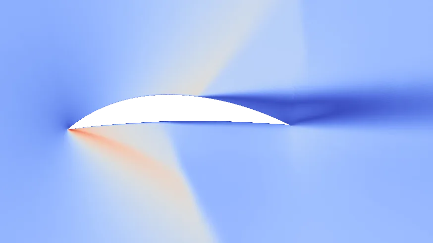
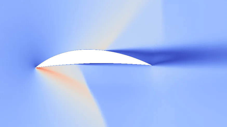
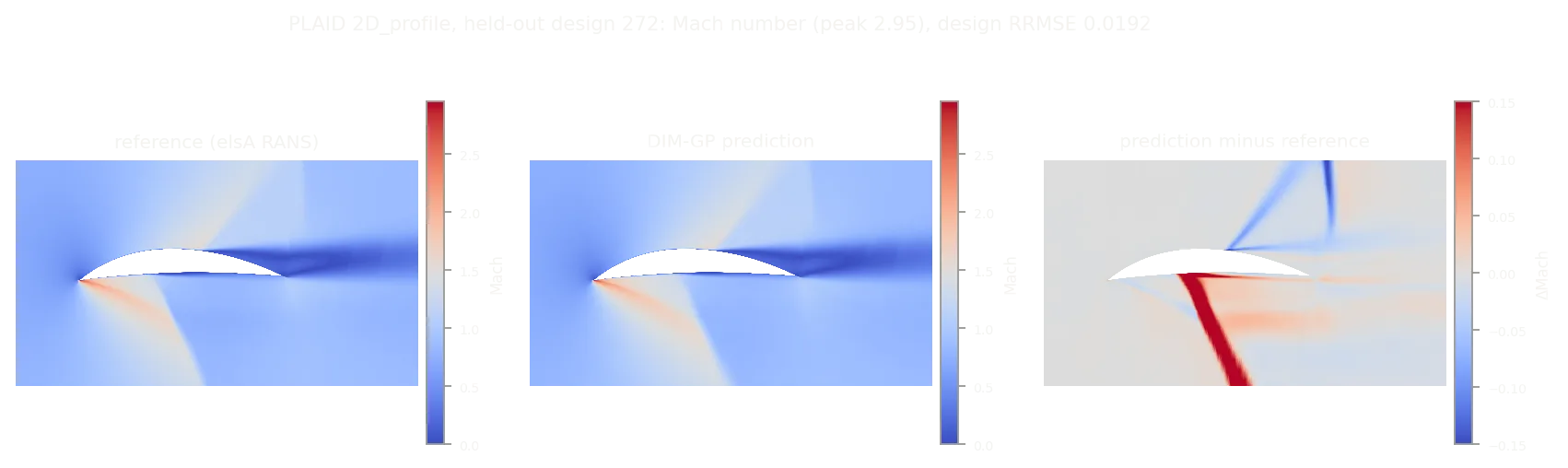
2D_profile [41] is the suite’s shape-only aerodynamics case: 300 training and 100 test airfoil profiles in a transonic flow, each with its own triangular mesh of 35,000–39,000 nodes cut close to the profile, and no input scalars at all — the geometry is the whole input, with the effective angle of attack baked into the shape. The competition scores four nodal fields (Mach number, pressure and the two velocity components). The test cases include transonic shocks.
Swipe or scroll horizontally to view all columns →
| RRMSE (lower is better) | Mach | Pressure | Velocity-x | Velocity-y | total |
|---|---|---|---|---|---|
| PXTransolver | 0.0134 | 0.0108 | 0.0155 | 0.0139 | 0.0134 |
| NPco | 0.0148 | 0.0097 | 0.0172 | 0.0136 | 0.0138 |
| DIM-GP | 0.0167 | 0.011 | 0.0196 | 0.0134 | 0.0152 |
| test-ts-dino | 0.0161 | 0.0114 | 0.0184 | 0.0149 | 0.0152 |
| Stest | 0.0168 | 0.0111 | 0.0198 | 0.0135 | 0.0153 |
| plaidtest | 0.0163 | 0.0111 | 0.0197 | 0.0146 | 0.0154 |
| Stealth | 0.0166 | 0.011 | 0.0195 | 0.0154 | 0.0157 |
| MM-GP+ | 0.0208 | 0.0139 | 0.0243 | 0.016 | 0.0187 |
| Transolver+ | 0.0209 | 0.0131 | 0.0267 | 0.019 | 0.0199 |
| test | 0.0211 | 0.0154 | 0.0242 | 0.0192 | 0.02 |
| Super MARIO | 0.022 | 0.0158 | 0.0251 | 0.0196 | 0.0206 |
| MARIO | 0.023 | 0.0146 | 0.0264 | 0.021 | 0.0213 |
| MeshFiLM | 0.0265 | 0.0177 | 0.0316 | 0.0243 | 0.025 |
| CRT | 0.0278 | 0.0171 | 0.0323 | 0.0244 | 0.0254 |
| MuFi-MiSe | 0.0279 | 0.018 | 0.0328 | 0.0315 | 0.0276 |
| MiSe-GNN | 0.0309 | 0.0212 | 0.0358 | 0.026 | 0.0285 |
| Vi-Transformer | 0.036 | 0.0167 | 0.0403 | 0.0307 | 0.0309 |
| MMGP | 0.0439 | 0.0208 | 0.0471 | 0.0342 | 0.0365 |
| Augur | 0.0469 | 0.0248 | 0.0538 | 0.0445 | 0.0425 |
| ICLGS | 0.0777 | 0.0248 | 0.0885 | 0.0601 | 0.0628 |
| FNO | 0.0988 | 0.0785 | 0.1148 | 0.0967 | 0.0972 |
| elzigomario | 0.1893 | 0.1004 | 0.2295 | 0.1199 | 0.1598 |
DIM-GP ranks third of 22 in the 7 September 2026 snapshot, with an aggregate error of 0.0152 versus PXTransolver’s 0.0134. The numerical gap is 0.0018, equivalent to 0.18 percentage points when these relative errors are expressed as percentages (1.52% versus 1.34%). DIM-GP’s Velocity-y error of 0.0134 is the lowest displayed value on the board; its pressure error of 0.011 is joint-third.
 referenceDIM-GP
Drag the slider: reference simulation on the left of the divider, DIM-GP prediction on the right (same colour scale). The three-panel figure below adds the difference map.
18. Bayesian optimization — concrete mix design, six approaches, one virtual problem
Bayesian optimization uses predictions and uncertainty estimates to select the next design to evaluate. Here, STOCHOS searches for concrete recipes that combine high 28-day compressive strength with low cradle-to-gate CO and material cost. Seven ingredient masses per cubic metre are varied, subject to a total mass of 2,195–2,551 kg.
The study uses a fixed virtual test bench fitted to the 1,022 usable rows of the public Concrete Compressive Strength dataset (UCI, 1,030 laboratory recipes) [45]. It predicts strength; CO and cost follow from the ingredient quantities, sourced emission factors and an indicative price basket. Six approaches receive the same starting recipes and a budget of 60 evaluations: STOCHOS, BoTorch’s qNEHVI [46], BayBE’s desirability approach [47], a random-forest optimizer, D-optimal design of experiments and random search.
Part A — reaching a specification. Five levels of increasing difficulty each demand a minimum strength together with a CO and a cost ceiling on the same recipe; difficulty is characterized by an estimated probability that a random valid recipe qualifies (1 in 9 for S1 down to 1 in 66,667 for S4.5), and an unreachable sixth level serves as a control that no method passes. Ten repeated runs per level, at round sizes of one, three and six recipes. The table counts, per level, how many of the 10 runs at one recipe per round found a qualifying recipe.
Choose the difficulty level to see how many runs met the strength, CO₂ and cost requirements as the experiment budget increased.
Swipe or scroll horizontally to view all columns →
| Runs that reached the specification (of 10) | S1 | S2 | S3 | S4 | S4.5 |
|---|---|---|---|---|---|
| STOCHOS | 10 | 10 | 10 | 10 | 10 |
| BoTorch (qNEHVI) | 10 | 10 | 10 | 10 | 8 |
| BayBE | 10 | 10 | 10 | 9 | 2 |
| Random forest | 10 | 10 | 7 | 3 | 1 |
| Classical DoE | 10 | 10 | 6 | 0 | 0 |
| Random search | 10 | 7 | 4 | 1 | 0 |
Over all five levels and all three round sizes STOCHOS reaches the specification in 149 of 150 runs, against 137 for BoTorch, 111 for BayBE, 87 for the random forest, 78 for classical DoE and 66 for random search; it is the only method that solves the extreme level in every sequential run. Among runs in which both STOCHOS and BoTorch succeeded, STOCHOS reached the target sooner in 99 of 136 comparisons, later in 16 and at the same experiment in 21 (reported two-sided sign test ).
Part B — discovering the trade-off set. With no single target, a method is scored on how much of the achievable trade-off region it discovers: the hypervolume of its evaluated recipes against a frozen reference point, averaged over 30 repeated runs; the table gives the coverage after 60 experiments at round sizes of one, five and ten.
Higher coverage means a broader set of useful trade-offs. Hover for exact values; error bars show the standard error across 30 runs.
Swipe or scroll horizontally to view all columns →
| Trade-off coverage after 60 experiments (hypervolume fraction) | 1 / round | 5 / round | 10 / round |
|---|---|---|---|
| STOCHOS | 0.9225 | 0.9150 | 0.8822 |
| BoTorch (qNEHVI) | 0.9105 | 0.9045 | 0.8917 |
| BayBE | 0.8900 | 0.8838 | 0.8726 |
| Random forest | 0.7740 | 0.7785 | 0.7679 |
| Classical DoE | 0.7345 | 0.7345 | 0.7345 |
| Random search | 0.6840 | 0.6840 | 0.6840 |
STOCHOS leads at round sizes one and five and is second at ten, where the batch of ten commits a sixth of the budget before any result returns. Choosing one recipe at a time, it reaches 80% coverage in a median of 32 experiments and 90% in 46 (on 20 of 30 runs, the most of any method); random forest, classical DoE and random search never reach 80% inside the budget. The extended-budget study of the classical design makes the gap concrete: a D-optimal plan needs 180 experiments to reach the 70% coverage that STOCHOS passes at 21.
Choose two objectives to compare the best trade-offs each method found across 30 runs. Higher strength, lower CO₂ and lower cost are preferred: towards the lower right in the strength views and towards the lower left in the CO₂–cost view.
Compare how many experiments each method needs to reach a given level of trade-off coverage. Higher curves indicate broader coverage at the same experiment budget.
Cost of the decisions. Part B’s sequential runs have median elapsed times of 26.7 minutes for STOCHOS, 50.2 minutes for BoTorch and 147.6 minutes for BayBE over 30 runs per method, each with a 60-experiment budget. STOCHOS uses approximately 47% less elapsed time than BoTorch in this comparison, measured for model fitting and proposal generation in the virtual benchmark. The methods with the lowest computational overhead, classical DoE and random search, have lower reported coverage.
Hover to see the time spent fitting models and proposing recipes. Compare the median computational time per campaign with the trade-off coverage above.
Appendix A. Sources and authorship
Public leaderboard rows, published baseline values and internal experiments are distinguished in the relevant sections. Numerical ranks refer to the stated comparison fields and snapshot dates. PLAID scores are computed by the benchmark platform; STOCHOS training and timing measurements are reported by the authors.
Swipe or scroll horizontally to view all columns →
| Material | Source | Licence / terms | Use in this report |
|---|---|---|---|
| TabArena code and published benchmark artifacts | AutoGluon [1] | Apache 2.0 | Reconstructed comparison and cited results |
| TALENT code and published results | LAMDA-Tabular [2] | MIT | Evaluation protocol and published comparison tables |
| PLAID datasets and leaderboard data | Safran [41] | CC BY-SA 4.0 | Evaluation, archived leaderboards and adapted visualizations |
| AhmedML | Ashton et al. [39] | CC BY-SA 4.0 | Evaluation and adapted visualizations |
| DrivAerML | Ashton et al. [43] | CC BY-SA 4.0 | Evaluation and adapted visualizations |
| LagrangeBench | Toshev et al. [33] | Dataset record and repository terms | Evaluation and adapted animations |
| Concrete Compressive Strength | Yeh / UCI [45] | CC BY 4.0 | Virtual optimization study |
| Water-3D and DeformingPlate | Google DeepMind [34, 48] | Source repository terms | Evaluation and author-created visualizations |
Adapted visualizations, predictions and annotations were produced by PI Probaligence GmbH. Visualizations adapted from PLAID, AhmedML and DrivAerML data are shared under CC BY-SA 4.0. The source datasets remain available under the terms linked above.
This report is authored by PI Probaligence GmbH, the developer of STOCHOS. References link to the benchmark datasets, published methods and evaluation protocols used in the comparisons.
References
References identify benchmark datasets, evaluation procedures, methods and author descriptions. For tabular entries, registered TabArena references were used where available.
Benchmarks
[1] TabArena: a living benchmark for tabular machine learning. Leaderboard https://huggingface.co/spaces/TabArena/leaderboard, code https://github.com/autogluon/tabrepo. Results accessed 18 August 2026 (42 registered methods).
[2] TALENT: a tabular analytics and learning toolbox. https://github.com/LAMDA-Tabular/TALENT.
Pretrained tabular models
[3] TabFM. Google Research, released 30 June 2026. https://github.com/google-research/tabfm. Released configuration: 1,639,444,298 parameters (§3). Consult the repository for license terms.
[4] EXAONE-Tabular. LG AI Research, released 31 July 2026. https://github.com/LGAI-Research/EXAONE-Tabular. Consult the repository for code and model-license terms.
[5] Prior Labs. TabPFN-3: Technical Report. arXiv:2605.13986. https://priorlabs.ai/technical-reports/tabpfn-3. Consult the model release for license terms.
[6] TabPFN-2.6 and RealTabPFN-2.5. arXiv:2511.08667.
[7] TabICL: a tabular foundation model for in-context learning on large data. arXiv:2502.05564. TabICLv2: arXiv:2602.11139. BSD-3-Clause.
[8] LimiX. arXiv:2509.03505.
[9] TabDPT. arXiv:2410.18164.
[10] Mitra. arXiv:2510.21204.
[11] TabPFN-Wide. arXiv:2510.06162.
[12] TabSTAR. arXiv:2505.18125.
[13] SAP-RPT-OSS. arXiv:2506.10707.
[14] OrionMSP. arXiv:2511.02818.
[15] iLTM. arXiv:2511.15941.
[16] Nori / Nori-30M. https://github.com/Synthefy/synthefy-nori.
[17] TabSwift. https://github.com/LAMDA-Tabular/TabSwift.
Trees, networks and classical baselines
[18] LightGBM: a highly efficient gradient boosting decision tree. NeurIPS 2017. https://papers.nips.cc/paper_files/paper/2017/hash/6449f44a102fde848669bdd9eb6b76fa-Abstract.html
[19] CatBoost: unbiased boosting with categorical features. arXiv:1706.09516.
[20] XGBoost: a scalable tree boosting system. arXiv:1603.02754.
[21] RealMLP — Better by default: strong pre-tuned MLPs and boosted trees on tabular data. arXiv:2407.04491.
[22] TabM. arXiv:2410.24210.
[23] ModernNCA. arXiv:2407.03257.
[24] xRFM. arXiv:2508.10053.
[25] Explainable Boosting Machine (EBM), Lou et al., KDD 2013.
[26] Random Forests, Breiman (2001), and Extremely Randomized Trees, Geurts et al. (2006).
[27] TorchMLP / FastaiMLP. arXiv:2003.06505.
[28] PerpetualBooster. https://perpetual-ml.com/.
Statistical methods used in this document
[29] R. A. Bradley and M. E. Terry. Rank analysis of incomplete block designs: I. The method of paired comparisons. Biometrika 39(3/4), 324–345 (1952). The model underlying the Elo ratings defined in §2.0.
[30] H. Theil (1950); P. K. Sen. Estimates of the regression coefficient based on Kendall’s tau. JASA 63(324), 1379–1389 (1968). The robust slope estimator used in §4.5.
[31] F. Wilcoxon. Individual comparisons by ranking methods. Biometrics Bulletin 1(6), 80–83 (1945). The paired test used in §4.2.
[32] J. Demšar. Statistical comparisons of classifiers over multiple data sets. JMLR 7, 1–30 (2006). On why paired, non-parametric tests are the appropriate instrument for benchmark comparisons of this shape.
Physics benchmarks and surrogate models (§§6–17)
[33] LagrangeBench: a Lagrangian fluid mechanics benchmarking suite. A. P. Toshev, G. Galletti, F. Fritz, S. Adami, N. A. Adams. NeurIPS 2023 Datasets & Benchmarks. arXiv:2309.16342. Datasets on Zenodo, CC-BY.
[34] Learning to simulate complex physics with graph networks (GNS). A. Sanchez-Gonzalez, J. Godwin, T. Pfaff, R. Ying, J. Leskovec, P. W. Battaglia. ICML 2020. arXiv:2002.09405. Source of the Water-3D dataset and protocol used in §8.
[35] Geometric and physical quantities improve E(3) equivariant message passing (SEGNN). J. Brandstetter, R. Hesselink, E. van der Pol, E. J. Bekkers, M. Welling. ICLR 2022 (spotlight). arXiv:2110.02905. Baseline in [33].
[36] CoRGI: convolutional residual global interactions. KDD 2026. arXiv:2511.22938. The strongest published per-cell numbers on most of the board in §7.2.
[37] Neural-SPH. arXiv:2402.06275. Source of the 400-step long-horizon protocol used in the supplement to §7.2.
[38] NeuralMPM. TMLR. arXiv:2408.15753. The only surveyed method reporting full-rollout MSE in the same convention as [34] (§8.2).
[39] AhmedML. N. Ashton et al. High-fidelity CFD dataset over the Ahmed body, 500 geometries. https://huggingface.co/datasets/neashton/ahmedml.
[40] AB-UPT: anchored-branched universal physics transformers. arXiv:2502.09692. Source of the baseline tables used in §§10.2 and 11. https://arxiv.org/abs/2502.09692.
[41] PLAID: a benchmark suite of physics-learning datasets. Safran. arXiv:2505.02974. Rotor37 leaderboard hosted at https://huggingface.co/PLAIDcompetitions. CC-BY-SA 4.0.
[42] EqGINO: equivariant geometry-informed Fourier neural operators for 3D PDEs. S. Kim, J. Song, S. Shin, G. Cho, S. Kim, C. Park. arXiv:2606.03260.
[43] DrivAerML: high-fidelity computational fluid dynamics dataset for road-car external aerodynamics. N. Ashton et al. arXiv:2408.11969. 500 morphed DrivAer variants, SA-sigma-DDES, ~160M cells; source of the solver-cost figures quoted in §11.
[44] Douglas Boubert. How an AI Agent Cracked an Industry Benchmark. PhysicsX, 11 August 2026. https://www.physicsx.ai/newsroom/how-an-ai-agent-cracked-an-industry-benchmark. Author description of the solver-based Tensile2d entry (§15).
[45] I-C. Yeh. Modeling of strength of high-performance concrete using artificial neural networks. Cement and Concrete Research 28(12), 1998. Dataset: UCI Machine Learning Repository, Concrete Compressive Strength (1,030 recipes).
[46] M. Balandat et al. BoTorch: A framework for efficient Monte-Carlo Bayesian optimization. NeurIPS 2020. botorch.org — qNEHVI acquisition, version 0.18.1 in §18.
[47] BayBE — Bayesian back end, Merck KGaA. emdgroup.github.io/baybe — version 0.15.0 in §18.
[48] T. Pfaff, M. Fortunato, A. Sanchez-Gonzalez, P. W. Battaglia. Learning mesh-based simulation with graph networks (MeshGraphNets). ICLR 2021. arXiv:2010.03409. Source of the DeformingPlate data and protocol of §9.
[49] M4GN: mesh-based multi-segment hierarchical graph network. Transactions on Machine Learning Research, 2025 (openreview.net/forum?id=R3vDbqWa1v). Reported 2.65 on DeformingPlate; no code released.
[50] MGN-T: MeshGraphNet-Transformer for solid mechanics. arXiv:2601.23177. DeformingPlate data regenerated with COMSOL.
[51] Y.-Y. Yu et al. Learning Flexible Body Collision Dynamics with Hierarchical Contact Mesh Transformer. ICLR 2024. https://arxiv.org/abs/2312.12467.
[52] Diffusion-Based Hierarchical Graph Neural Networks for Simulating Nonlinear Solid Mechanics (ROBIN). NeurIPS 2025. https://arxiv.org/abs/2506.06045.
[53] EvoMesh: Adaptive Physical Simulation with Hierarchical Graph Evolutions. ICML 2025. https://hbell99.github.io/evo-mesh/.
[54] Y. Cao, M. Chai, M. Li and C. Jiang. Efficient Learning of Mesh-Based Physical Simulation with Bi-Stride Multi-Scale Graph Neural Network. ICML 2023. https://proceedings.mlr.press/v202/cao23a.html.
[55] A. Vaswani et al. Attention Is All You Need. NeurIPS 2017. https://arxiv.org/abs/1706.03762.
[56] H. Wu et al. Transolver: A Fast Transformer Solver for PDEs on General Geometries. ICML 2024. https://arxiv.org/abs/2402.02366.
[57] Z. Li et al. Transformer for Partial Differential Equations’ Operator Learning. ICLR 2023. https://arxiv.org/abs/2205.13671.
[58] B. Alkin et al. Universal Physics Transformers: A Framework For Efficiently Scaling Neural Operators. NeurIPS 2024. https://arxiv.org/abs/2402.12365.
[59] H. Gao and S. Ji. Graph U-Nets. ICML 2019. https://arxiv.org/abs/1905.05178.
[60] Z. Li et al. Geometry-Informed Neural Operator for Large-Scale 3D PDEs. NeurIPS 2023. https://arxiv.org/abs/2309.00583.
[61] C. R. Qi et al. PointNet: Deep Learning on Point Sets for 3D Classification and Segmentation. CVPR 2017. https://arxiv.org/abs/1612.00593.
[62] T. Wang and C. Wang. Latent Neural Operator for Solving Forward and Inverse PDE Problems. NeurIPS 2024. https://arxiv.org/abs/2406.03923.
[63] PI Probaligence. How STOCHOS Works: The DIM-GP Algorithm. Technical description (not a peer-reviewed method paper). https://probaligence.com/how-stochos-works/.
[64] NVIDIA. NVIDIA H100 Tensor Core GPU. Product specifications, including H100 SXM memory bandwidth and Tensor performance. https://www.nvidia.com/en-us/data-center/h100/.
[65] NVIDIA. NVIDIA H100 Tensor Core GPU PCIe Product Brief. Product specifications, including H100 PCIe memory bandwidth and Tensor performance. https://www.nvidia.com/content/dam/en-zz/Solutions/gtcs22/data-center/h100/PB-11133-001_v01.pdf.
[66] NVIDIA. NVIDIA Ada GPU Architecture. GeForce RTX 4090 specifications, including memory bandwidth and Tensor performance. https://images.nvidia.com/aem-dam/Solutions/geforce/ada/nvidia-ada-gpu-architecture.pdf.