

What the model had to predict
ZF was after the fatigue life of solder joints on a ball grid array component, the usual failure point in automotive electronics under thermal cycling. The physics of failure route is a nonlinear creep simulation, and it costs enough that the analysis normally stops at the component itself. The board, the neighbouring components, and how the assembly is mounted get left out, and the study is direct about the cost: the simulated life can come out badly distorted.
The method under test replaces that nonlinear step with a surrogate. Displacements at the solder ball's connecting faces go in, accumulated creep strain in the ball comes out. That trades one problem for another: the deformation has to be described by a manageable set of inputs, and the more of them you keep, the more faithful the description and the harder the model is to fit. ZF ran the comparison at three input dimensions, 22, 46, and 94 free parameters.
How the comparison was set up
Every training sample is a nonlinear FE run. So the question is not which method fits best given unlimited data. It is which method reaches a usable model on the smallest simulation budget.
The baseline is Latin hypercube sampling: spread the samples evenly across the input space up front, then fit. Adaptive sampling works in rounds instead. Both adaptive runs here are built on 100 LHS points and add 10 samples per iteration, placing them where the model's coverage is thin rather than everywhere at once. PI-BO makes that choice probabilistically, using the model's own uncertainty to find where the next simulation is worth running.
Two metrics, both measured on held-out test data. R squared is the share of the variance the model explains, and the study treats above 0.9 as high explanatory power and below 0.5 as only marginally suited to prediction. MAPE is the mean absolute percentage error, so lower is better.
What the numbers show
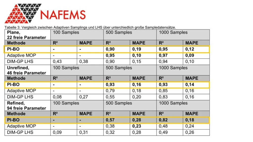
Read the table above from the bottom block upward and the pattern is consistent: the harder the problem, the more the sampling strategy decides the outcome.
At 94 free parameters, evenly spread sampling reaches R squared 0.49 at 1000 samples, below the study's own 0.5 line for a model worth predicting with. PI-BO reaches 0.82 on the same 1000 samples, with MAPE down from 0.26 to 0.18. Same simulation budget, and the model crosses from marginal to usable.
At 46 free parameters, PI-BO reaches 0.93 at 500 samples. Even sampling is still at 0.83 with twice as many, 1000. Better model, half the runs.
At 22 free parameters, there is little left to win. Plain LHS already reaches 0.94 by 1000 samples and PI-BO ends at 0.95. That is the useful part of the result: adaptive sampling earns its keep once the input space is large enough that spreading points evenly stops covering what matters.
What it means if you are choosing a sampling strategy
The cost of a surrogate is not the fitting, it is the runs you have to pay for to train it. Even sampling spends that budget before it knows anything about the response. Adaptive sampling spends most of it after, which is why the gap opens up exactly where the budget is tightest relative to the size of the problem.
The rule that falls out of ZF's three blocks: in low dimensions, plain LHS is fine and simpler. Above that, the same number of simulations buys a materially better model if you place them adaptively. ZF's own conclusion from the study was that PI-BO is the one to reach for on high dimensional problems.
That is the case PI-BO is built for. It sits on the same probabilistic engine as the rest of STOCHOS, so the uncertainty it uses to choose the next sample is the uncertainty the finished surrogate model reports back to you.
Where to read the study
The full paper, "Maschinelles Lernen gestützte Modellbildung für kriechdehnungsbasierte Lebensdaueranalyse einer Ball Grid Array Komponente" by Markus Tauscher (ZF Friedrichshafen) and Jürgen Wilde (Universität Freiburg), is in the proceedings of the NAFEMS seminar on artificial intelligence and machine learning in CAE-based simulation. The proceedings are available to NAFEMS members through the NAFEMS resource centre.
It meant a lot that a partner chose to put the method in front of that audience.
Learn more: how STOCHOS combines surrogate modeling with uncertainty quantification for reliable engineering predictions.